Gas well deliverability

The gas plant will be sized for a contracted throughput, and the gas sales contract will commit Prairie Crest to deliver it. That makes deliverability, the rate a well can produce against a given back-pressure, the link between the reservoir and the money. Farid starts Ethan on the Oriskany sandstone pool's best well, C-4, which has just completed a modified isochronal test. “An oil engineer would draw a straight-line IPR and call it a day,” Farid says. “Gas wells are not straight lines. Part of the pressure drop goes into turbulence near the wellbore, and it grows with the square of the rate.”

Radial flow of gas

Darcy's law for steady radial flow of an oil leads to a productivity index: rate proportional to drawdown. For gas, the density and viscosity change with pressure, and the mass rate, not the volume rate, is constant along the flow path. Integrating Darcy's law with the real-gas law at constant temperature gives, for pseudo-steady-state flow in field units:

Here q_g is in Mscf/d, k in millidarcies, h in feet, pressures in psia, T in °R and μ in centipoise; μ̄ and z̄ are evaluated at an average pressure. The pressure-squared form is accurate below about 2,000 to 3,000 psia, where μz is nearly constant. At higher pressures, where p/(μz) is nearly constant instead, a linear pressure form works better, and the exact approach uses the pseudo-pressure of Lesson 6, which is valid at all pressures.

The term D q_g is the rate-dependent skin. Near the wellbore the gas velocity is high, and the pressure drop includes an inertial component proportional to the square of the velocity, described by Forchheimer's extension of Darcy's law. Engineers call it non-Darcy or turbulent flow, although true turbulence is not required. Because it appears as an extra skin proportional to rate, a gas well's apparent skin rises with rate, and doubling the drawdown less than doubles the rate.

The back-pressure equation

Long before the theory was settled, Rawlins and Schellhardt of the US Bureau of Mines (1935) found empirically that gas well rates fitted a simple power law:

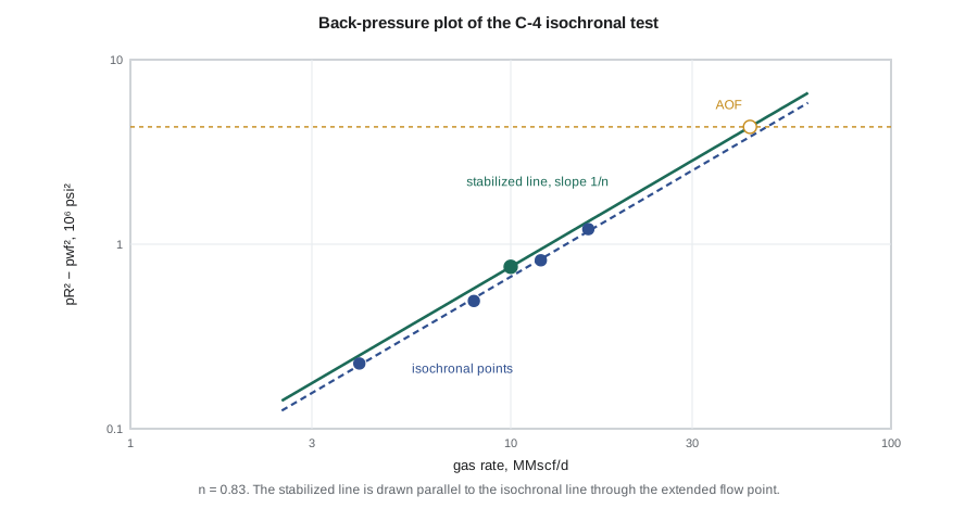
On a log-log plot of p̄² − p_wf² against q_g the test points fall on a straight line with slope 1/n. The exponent n ranges from 1 for pure Darcy flow to 0.5 for fully inertial flow; most wells fall between 0.6 and 0.9. The constant C depends on the flow time until the drainage radius reaches the boundary, after which it stabilizes. The absolute open flow potential, AOF, is the rate the equation predicts at zero flowing bottomhole pressure. No well actually flows at zero pressure, but the AOF is a standard way to compare wells, and regulators commonly require it.

The laminar-inertial-turbulent equation

The back-pressure equation is convenient but inexact: n is not truly constant, and extrapolating it beyond the tested rates can overstate the AOF. The laminar-inertial-turbulent, or LIT, equation follows directly from the Forchheimer form of the radial flow equation:

The coefficient a contains the Darcy terms, including the mechanical skin, and b the non-Darcy coefficient D. Plotting (p̄² − p_wf²)/q_g against q_g gives a straight line with slope b and intercept a. Houpeurt (1959) wrote the same equation in pseudo-pressure, Δm = a q + b q², which removes the low-pressure limitation. For high-rate wells the LIT analysis is preferred, and its AOF follows from solving the quadratic at p_wf = 0.

Deliverability test types

A flow-after-flow test, the original method, flows the well at three or four increasing rates, each until the pressure stabilizes, without shut-ins between. In permeable rock this takes hours; in tighter rock, stabilization can take days or weeks for each rate, and the gas must be flared or sold. The isochronal test, introduced by Cullender in 1955, avoids long stabilization by flowing each rate for the same short time, with a shut-in to near-average pressure between flows, and then one extended flow to stabilization. The short flows all reach the same radius of investigation, so they define the slope (n or b), and the extended flow fixes the stabilized C or a. The modified isochronal test shortens the shut-ins to equal the flow periods and uses the last shut-in pressure before each flow in place of the average pressure. It is the most common test today because it is cheap, and its error is small unless the shut-ins are very short in a tight well.

# Deliverability of the C-4 gas well: Rawlins-Schellhardt back-pressure fit (C and n)
# and the laminar-inertial-turbulent (LIT) fit, with the absolute open flow and an IPR table.
import math
SI = False     # True: metric units, False: oilfield units

pR = 2080.0                                   # average reservoir pressure, psia
# isochronal test: (rate MMscf/d, flowing bottomhole pressure psia); the last point is the extended flow
test = [(4.0, 2025.0), (8.0, 1958.0), (12.0, 1873.0), (16.0, 1766.0)]
ext = (10.0, 1890.0)

def fit(xs, ys):
    n = len(xs); mx, my = sum(xs) / n, sum(ys) / n
    b = sum((x - mx) * (y - my) for x, y in zip(xs, ys)) / sum((x - mx) ** 2 for x in xs)
    return b, my - b * mx

dp2 = [pR ** 2 - p ** 2 for q, p in test]
# back-pressure equation q = C (pR^2 - pwf^2)^n, slope from the isochronal points
n_bp, lnC = fit([math.log(d) for d in dp2], [math.log(q) for q, p in test])
C = ext[0] / (pR ** 2 - ext[1] ** 2) ** n_bp     # stabilized C through the extended point
aof_bp = C * pR ** (2 * n_bp)
# LIT equation pR^2 - pwf^2 = a q + b q^2: b from the isochronal points, a from the extended point
b, a_iso = fit([q for q, p in test], [d / q for d, (q, p) in zip(dp2, test)])
a = ((pR ** 2 - ext[1] ** 2) - b * ext[0] ** 2) / ext[0]
aof_lit = (-a + math.sqrt(a * a + 4 * b * pR ** 2)) / (2 * b)
k2, k3 = 28.3168e-3, 0.145038                 # 10^6 m3 per MMscf and psi per kPa
print(f"Back-pressure: n = {n_bp:.3f}")
if SI:
    u = (1 / k3) ** 2                             # kPa2 per psi2
    print(f"LIT: a = {a * u / 28.3168:,.0f} kPa2 per 10^3 m3/d, b = {b * u / 28.3168 ** 2:,.1f} kPa2 per (10^3 m3/d)2")
    print(f"AOF back-pressure {aof_bp * k2 * 1000:,.0f} 10^3 m3/d, LIT {aof_lit * k2 * 1000:,.0f} 10^3 m3/d")
    print(" pwf kPa   q back-pressure   q LIT   (10^3 m3/d)")
else:
    print(f"LIT: a = {a:,.0f} psi2 per MMscf/d, b = {b:,.0f} psi2 per (MMscf/d)2; isochronal a = {a_iso:,.0f}")
    print(f"AOF back-pressure {aof_bp:.1f} MMscf/d, LIT {aof_lit:.1f} MMscf/d")
    print(" pwf psia  q back-pressure   q LIT   (MMscf/d)")
for frac in [0.9, 0.75, 0.6, 0.45, 0.3, 0.0]:
    pwf = frac * pR; d = pR ** 2 - pwf ** 2
    q1 = C * d ** n_bp
    q2 = (-a + math.sqrt(a * a + 4 * b * d)) / (2 * b)
    if SI: print(f"{pwf / k3:8,.0f}  {q1 * k2 * 1000:12,.0f}  {q2 * k2 * 1000:10,.0f}")
    else: print(f"{pwf:8,.0f}  {q1:12.1f}  {q2:10.1f}")
print(f"Share of drawdown lost to non-Darcy flow at the extended rate: {b * ext[0] ** 2 / (a * ext[0] + b * ext[0] ** 2):.0%}")

Back-pressure: n = 0.830
LIT: a = 59,502 psi2 per MMscf/d, b = 1,593 psi2 per (MMscf/d)2; isochronal a = 49,495
AOF back-pressure 42.6 MMscf/d, LIT 36.7 MMscf/d
 pwf psia  q back-pressure   q LIT   (MMscf/d)
   1,872          10.7        10.7
   1,560          21.5        20.5
   1,248          29.4        27.0
     936          35.3        31.5
     624          39.4        34.4
       0          42.6        36.7
Share of drawdown lost to non-Darcy flow at the extended rate: 21%

The back-pressure fit gives n = 0.83 and an AOF of about 42.6 MMscf/d. The LIT fit gives an AOF of about 36.7 MMscf/d. The difference comes from the extrapolation: the back-pressure line assumes a constant n, while the LIT quadratic lets the non-Darcy term grow with the square of the rate. At the rates the well will actually produce, 10 to 20 MMscf/d, the two agree within 5 percent. At the extended rate of 10 MMscf/d, about a fifth of the drawdown already goes into non-Darcy flow, a sign that the near-well region would repay attention: more perforations or a larger completion interval would reduce the gas velocity at the sandface.

Inflow performance and the tubing

The inflow performance relationship (IPR) from the test gives the rate at each bottomhole flowing pressure. The well's actual rate is where the IPR meets the tubing performance curve, which gives the bottomhole pressure needed to lift a given rate to the surface against the wellhead pressure. For gas wells, the tubing curve comes from the static gas column, which is substantial at 6,500 ft or more, and friction, which rises steeply with rate in small tubing. The gathering system adds its own back-pressure at the wellhead. Nodal analysis, which the production course covered, finds the operating point and shows which component is the bottleneck. For C-4 it is the 2⅞-inch tubing at rates above about 14 MMscf/d: larger tubing would add rate today, but would load up with water earlier as the reservoir depletes.

Liquid loading

That trade-off is a central issue of gas well operations. A gas well always produces some liquid, condensed water and condensate, and the gas must carry it up the tubing. Turner and others (1969) showed that a well unloads liquid only if the gas velocity exceeds a critical velocity, set by the largest droplet that can be suspended against gravity. Below it, liquid falls back, accumulates and adds hydrostatic back-pressure, the rate falls further and the well can die. The critical rate is proportional to the tubing area and roughly to the square root of the pressure. As reservoir pressure declines, operators lower wellhead pressure with compression, install smaller tubing (velocity strings), use plunger lift or foamers, or install artificial lift. In the Marcellus, where wells start at very high rates and decline quickly, liquid loading appears within a few years and is a design input from the start.

Deliverability over time

The stabilized IPR describes one moment. As the reservoir depletes, p̄ falls and the whole curve shifts down; C stays roughly constant for a well in boundary-dominated flow, so the AOF falls with p̄^(2n). The development plan forecasts each well's deliverability year by year from the material balance pressure and the back-pressure or LIT equation, checks it against the plant's demand and the gathering pressures, and adds compression or new wells when the field can no longer meet the contract. Ethan builds such a forecast for the Oriskany sandstone pool: with today's gathering pressure the pool's six wells can hold 90 MMscf/d for about three more years; with a wellhead compressor lowering the suction pressure, plateau extends by about two years.