
PET-380 · Lesson 7 of 12 · 19 min
Empirical correlations
Back in the facilities group, Sofia gives Ethan a table from the field data system: two years of daily rates, inlet and outlet pressures on the north pad line, and the elevation profile from the as-built survey. 'Our design software offers a dozen correlations,' she says. 'Each one gives a different answer. Your job is to find out which ones describe this line, and why the others do not.' Tom Ashworth, the reservoir engineer, adds a request of his own: 'When you are done, tell me which one I should use in the integrated model for the Birch Coulee gas pool wells too.'
This lesson surveys the main empirical correlations for multiphase pressure drop, explains how they were developed and what data they rest on, works through the Beggs and Brill method in detail, and shows how to compare correlations against field measurements and choose among them.
What an empirical correlation is
An empirical correlation is a set of equations fitted to experimental or field data, usually expressed in dimensionless groups, that predicts holdup and friction without modeling the detailed physics of each flow pattern. The developers measured pressure gradients, and in some cases holdup, over a range of rates, pipe sizes and fluids, then chose a functional form and fitted its coefficients. The result can be very accurate within the range of its data and unreliable outside it.
Brill and Mukherjee, in their 1999 SPE monograph on multiphase flow in wells, grouped correlations into three categories. Category A methods assume no slip and no flow pattern distinctions; they predict only a friction factor. Category B methods account for slip, with a holdup correlation, but do not distinguish flow patterns. Category C methods account for both slip and flow patterns. The categories help explain why older methods fail in some conditions: a category A method cannot capture the high holdup of slow uphill flow, however carefully its friction factor is fitted.
The main correlations
Poettmann and Carpenter, in 1952, published one of the first methods for oil wells, a category A correlation based on a fitted energy-loss factor from 49 flowing and gas-lift wells. It works only for the high-rate, small-tubing conditions it was drawn from.
Hagedorn and Brown, in 1965, used a 1,500 ft (457 m) experimental well at the University of Texas to measure pressure gradients for a range of rates, tubing sizes and liquid viscosities. Their holdup correlation, a category B method, was obtained by working backward from the measured gradients. In its original form it can predict holdup below the no-slip fraction, which is physically impossible, so most software applies the correction that holdup must be at least λ_L, together with the Griffith bubble-flow correction. Modified Hagedorn-Brown remains one of the most reliable correlations for vertical oil wells.
Duns and Ros, whose flow pattern map was introduced in lesson 5, used their laboratory data to build a category C method for vertical flow, with separate slip and friction equations for each region. It performs well in gas-condensate and high gas-liquid ratio wells, and less well in some oil wells.
Orkiszewski, in 1967, combined the Griffith-Wallis method for bubble flow, his own method for slug flow, and Duns-Ros for transition and mist flow, choosing the pieces that best matched a set of 148 field wells. Aziz, Govier and Fogarasi, in 1972, developed a more mechanistic approach to vertical bubble and slug flow, and their method is often considered a bridge between empirical and mechanistic models.
For horizontal and inclined pipes, Lockhart and Martinelli's 1949 method expressed the two-phase friction gradient as a multiplier on the single-phase gradient of either phase, correlated against a parameter X, the square root of the ratio of liquid-alone to gas-alone gradients. Dukler, in 1964, developed a similarity-based method for horizontal pipelines that is still used for gas-condensate lines, often with the Eaton holdup correlation, which was based on field-scale tests in 2-inch and 4-inch lines. Mukherjee and Brill, in 1985, used an inclinable U-shaped test loop to develop a correlation for all inclinations, with flow pattern dependent holdup.
Beggs and Brill
Beggs and Brill developed their correlation in 1973 from experiments in 1-inch and 1.5-inch acrylic pipes, 90 ft (27 m) long, that could be inclined at any angle from −90 to +90 degrees. They used air and water and measured holdup directly with quick-closing valves. Because it covers all inclinations, it became a standard for pipelines and deviated wells, and it is still the default in much software, usually with later modifications.
The method works in four stages. First, the horizontal flow pattern is found from the Froude number and λ_L, as in lesson 4. Second, the horizontal holdup is calculated from a power-law expression whose coefficients depend on the pattern:
Third, the holdup is corrected for inclination with a factor ψ that depends on the angle and on a coefficient C, itself a function of λ_L, the liquid velocity number and the Froude number:
The factor ψ peaks at about 50 degrees uphill, reflecting the experimental observation that holdup in upward flow is largest at moderate inclinations. Fourth, the two-phase friction factor is obtained by multiplying the no-slip friction factor by an exponential function of a parameter y = λ_L / H_L². In the transition zone, holdup is interpolated between the segregated and intermittent values.
Several later modifications are common. Later workers, including Palmer in 1975 and Payne and coworkers in 1979, found that the original method overpredicts holdup in inclined flow and proposed multipliers on the calculated holdup; the factors usually applied in software are about 0.924 for uphill flow and 0.685 for downhill flow. Many programs use a revised Beggs-Brill that adds a stratified smooth pattern, uses a rough-pipe friction factor rather than the smooth-pipe one of the original paper, and applies the holdup floor H_L ≥ λ_L.
# Beggs-Brill liquid holdup with the inclination correction (coefficients from the 1973 paper, as usually tabulated)
import math
SI = False
g = 9.81
H0 = {"segregated": (0.98, 0.4846, 0.0868), "intermittent": (0.845, 0.5351, 0.0173), "distributed": (1.065, 0.5824, 0.0609)}
UP = {"segregated": (0.011, -3.768, 3.539, -1.614), "intermittent": (2.96, 0.305, -0.4473, 0.0978)}
def holdup(pat, lam, NFr, NLv, theta_deg):
    a, b, c = H0[pat]
    h0 = max(a * lam ** b / NFr ** c, lam)
    if pat == "distributed" or theta_deg == 0: return h0
    e, f, gg, h = UP[pat]
    C = max(0.0, (1 - lam) * math.log(e * lam ** f * NLv ** gg * NFr ** h))
    th = math.radians(theta_deg)
    psi = 1 + C * (math.sin(1.8 * th) - math.sin(1.8 * th) ** 3 / 3)
    return h0 * psi
D, vsl, vsg = 0.154, 0.12, 0.72
rhoL, sig = 880.0, 0.028
vm = vsl + vsg; lam = vsl / vm; NFr = vm * vm / (g * D)
NLv = vsl * (rhoL / (g * sig)) ** 0.25
print(f"lambda_L {lam:.3f}, Froude {NFr:.3f}, liquid velocity number {NLv:.3f}")
for th in (0, 2, 5, 10):
    H = holdup("segregated", lam, NFr, NLv, th)
    rhos = rhoL * H + 15.0 * (1 - H)
    grad = rhos * g * math.sin(math.radians(th)) / 1000
    if SI: print(f"uphill {th:2d} deg: holdup {H:.3f}, elevation gradient {grad:5.2f} kPa/m")
    else:  print(f"uphill {th:2d} deg: holdup {H:.3f}, elevation gradient {grad * 0.145038 * 0.3048:5.3f} psi/ft")
# Error band: a correlation that is 20 percent wrong on holdup moves the elevation term by the same fraction
H = holdup("segregated", lam, NFr, NLv, 5)
for err in (-0.2, 0.2):
    Hx = H * (1 + err); rhos = rhoL * Hx + 15 * (1 - Hx)
    dp = rhos * g * 60.0 / 1000                       # 60 m of net climb
    print(f"holdup {err:+.0%}: elevation loss over a 60 m climb {dp:5.0f} kPa" if SI else
f"holdup {err:+.0%}: elevation loss over a 197 ft climb {dp * 0.145038:5.1f} psi")lambda_L 0.143, Froude 0.467, liquid velocity number 0.903 uphill 0 deg: holdup 0.408, elevation gradient 0.000 psi/ft uphill 2 deg: holdup 0.489, elevation gradient 0.007 psi/ft uphill 5 deg: holdup 0.608, elevation gradient 0.020 psi/ft uphill 10 deg: holdup 0.794, elevation gradient 0.053 psi/ft holdup -20%: elevation loss over a 197 ft climb 37.2 psi holdup +20%: elevation loss over a 197 ft climb 55.1 psi
Ethan's results show the holdup rising from about 0.41 on flat ground to nearly 0.8 on a 10-degree climb. The second part of the output makes Sofia's point for her: a 20 percent error in holdup moves the elevation loss over the line's steepest 197 ft climb by about 18 psi. 'For a gravity-dominated line,' she says, 'the holdup model is the design. Everything else is detail.'
Comparing correlations against field data
No correlation is best everywhere. Published comparisons, including the large data-bank studies carried out in the 1980s and 1990s, generally found errors of 10 to 30 percent in pressure drop for the better methods, and much more for some methods outside their range. The only reliable way to choose a correlation for a given field is to test it against measured data from that field.
A good comparison uses several periods with different rates, accurate pressure gauges at both ends of the line, an accurate elevation profile, and representative fluid properties. For each test the engineer computes the predicted pressure drop and the error. Two statistics summarize the results. The average percent error shows bias, whether the method tends to overpredict or underpredict. The average absolute percent error, or the standard deviation of the percent error, shows scatter. A method with small bias and small scatter is preferred; a method with small scatter but consistent bias can sometimes be tuned with a single multiplier on holdup or friction.
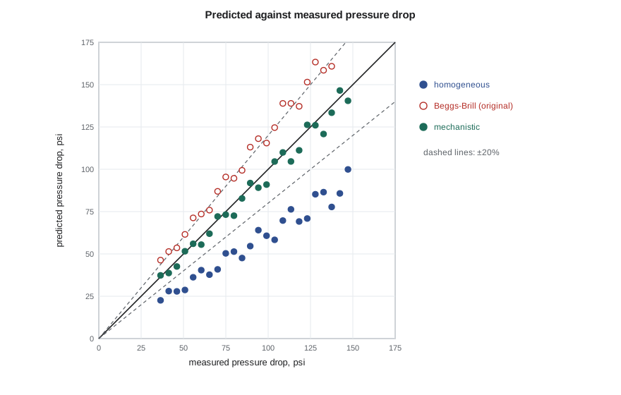
| Method | Average error | Average absolute error | Points within ±20% |
|---|---|---|---|
| Homogeneous | −38% | 38% | 4 of 24 |
| Beggs-Brill (original) | +22% | 24% | 11 of 24 |
| Beggs-Brill with holdup multipliers | +6% | 13% | 19 of 24 |
| Mechanistic (lesson 8) | −3% | 9% | 22 of 24 |
Ethan's results follow the pattern described in the literature. The homogeneous model underpredicts badly, because the line is dominated by uphill holdup. The original Beggs-Brill overpredicts, consistent with the published findings. The corrected version and the mechanistic model both perform well. Sofia asks him to keep both and to see which tracks the declining rates better over the next year. Tom gets his answer too: for the gas wells, where liquid loading near the critical rate matters most, Ethan recommends a mechanistic model checked against the wells' own rate tests.
Choosing a correlation
Experience suggests some general guidance, always to be checked against field data. For vertical oil wells, modified Hagedorn-Brown is a sound starting point. For gas-condensate and high gas-liquid ratio wells, Duns-Ros or a mechanistic model often performs better. For deviated wells and pipelines on hilly terrain, a method that handles inclination explicitly, such as Beggs-Brill with modifications or Mukherjee-Brill, is needed, and mechanistic models usually do better still. For long, nearly horizontal gas-condensate lines, Dukler-Eaton or a mechanistic method is common. Whatever method is chosen, its range of development data should cover the pipe size, rates and fluid properties of the case at hand, and its predictions should be compared with at least a few field measurements before it is used for design.
Tuning and its risks
When a correlation shows a consistent bias, engineers often tune it with a multiplier on holdup or friction so that it matches the field data. Tuning is reasonable if the bias is consistent across rates and the line will operate in a similar range. It is risky if the correlation is matched at high rates and then used for late-life low rates, because the dominant term may change from friction to gravity, and a friction multiplier will not correct a holdup error. A tuned model should be re-checked whenever rates or fluids change substantially, and the tuning factors should be recorded so that later users know what was done.
Worked problem
Bias and scatter
Four test periods give measured pressure drops of 400, 520, 610 and 700 units, and a correlation predicts 440, 560, 650 and 720 units. Find the average percent error and the average absolute percent error.
Show solution
- Percent errors: (440 − 400)/400 = +10.0%; (560 − 520)/520 = +7.7%; (650 − 610)/610 = +6.6%; (720 − 700)/700 = +2.9%.
- Average percent error: (10.0 + 7.7 + 6.6 + 2.9)/4 = +6.8%.
- Because all errors are positive, the average absolute percent error is also 6.8%.
Answer: The method has a consistent overprediction of about 7 percent with little scatter, so a single holdup multiplier near 0.93 could reasonably be tried.
Common mistakes
MistakeChoosing a correlation because it is the software default.
InsteadTest candidate methods against field data from the line or a similar one.
MistakeUsing a vertical well correlation for an inclined pipeline.
InsteadUse methods developed or tested for the relevant inclinations.
MistakeTuning friction to fix a holdup error.
InsteadIdentify the dominant term; tune the term that is wrong.
MistakeExtrapolating far beyond the correlation's data range.
InsteadCheck pipe size, rates and fluids against the development data.
Summary and key terms
- Empirical correlations fit equations in dimensionless groups to experimental or field data.
- Methods are grouped by whether they account for slip and flow patterns (categories A, B and C).
- Hagedorn-Brown (modified) is widely used for vertical oil wells; Beggs-Brill for all inclinations.
- Beggs-Brill finds the pattern, calculates horizontal holdup, corrects for inclination and adjusts the friction factor.
- Correlations are compared against field data using bias (average error) and scatter (absolute error).
- Tuning can remove bias but is risky when the dominant term changes.
- Empirical correlation
- A set of equations fitted to measured data rather than derived from detailed physics.
- Inclination correction
- A factor that adjusts horizontal holdup for the pipe angle.
- Bias
- The average signed error of a method, showing systematic over- or underprediction.
- Scatter
- The spread of errors about the average, often measured by the absolute error.
- Tuning
- Adjusting a model with a multiplier so that it matches measured data.
- Lockhart-Martinelli parameter
- The square root of the ratio of liquid-alone to gas-alone friction gradients.
Practice problems
Work each problem on paper first, then reveal the answer to check.
What distinguishes category C correlations?
Show answer
They account for both slip and flow patterns.
Why are holdup multipliers often applied to Beggs-Brill?
Show answer
The original method overpredicts holdup in inclined flow.
What two statistics are used to compare correlations?
Show answer
Average percent error (bias) and average absolute percent error (scatter).
Why can tuning a friction multiplier mislead at late-life rates?
Show answer
Gravity may dominate at low rates, so a friction multiplier does not fix the holdup error.
Lesson quiz · 5 questions
Score 60% or more to complete this lesson.
Create a free account to save your progress, take quizzes and earn a certificate.