Single-phase pipe flow review

Before he tackles gas and liquid together, Sofia asks Ethan to refresh the single-phase tools that every multiphase method is built on. 'Every correlation you will meet,' she says, 'ends up calling a friction factor and a gravity term somewhere inside. If you do not trust your single-phase numbers, you cannot trust the multiphase ones.' She gives him two problems from the gathering system: a produced-water line that carries only liquid, and the 4-inch gas line from the Birch Coulee gas pool that runs to the compressor station.

This lesson reviews the energy balance for steady flow in a pipe, the Reynolds number and the friction factor, the Moody chart and the Colebrook equation, minor losses, and the special forms of the equations used for long gas lines. These ideas were covered in fluid mechanics; here they are applied to petroleum pipelines and prepared for use in multiphase calculations.

The pressure gradient equation

For steady flow in a pipe of constant diameter, a momentum balance on a short segment gives the pressure gradient as the sum of three parts: the weight of the fluid, wall friction and the change in kinetic energy.

Here p is pressure, L distance along the pipe, ρ the fluid density, g gravity, θ the angle of the pipe above horizontal, f the Darcy friction factor, v the average velocity and D the inside diameter. In a horizontal liquid line only the friction term remains. In a vertical liquid well the gravity term usually dominates. The acceleration term is small for liquids and for most gas lines, but it matters near the outlet of a high-velocity gas line, where pressure falls quickly and the gas expands.

The same three terms appear in every multiphase method. What changes is how the density and velocity of the mixture are defined, and how the friction factor is calculated when two phases share the wall.

Reynolds number and flow regime

The Reynolds number compares inertial and viscous forces:

Below about 2,000 to 2,300 the flow is laminar and the friction factor is 64/Re. Above about 4,000 it is turbulent, and the friction factor depends on both Re and the relative roughness ε/D. Between the two is a transition zone where the friction factor is uncertain. Most petroleum pipelines operate in turbulent flow, but heavy oils, cold emulsions and low-rate lines can be laminar, and wrongly assuming turbulence then underestimates the pressure drop at low rates.

Friction factor: Moody and Colebrook

For turbulent flow in commercial pipe, the Colebrook equation relates the friction factor to Reynolds number and relative roughness:

Because f appears on both sides, the equation is solved by iteration, starting from a guess such as 0.02. Explicit approximations avoid the iteration. The Swamee-Jain equation is accurate to within about one percent over most of the practical range, and is often used in spreadsheets and in the inner loops of multiphase software:

The Moody chart is a plot of these relationships. At high Reynolds number and rough pipe the curves become flat: friction depends only on roughness, and the pressure drop rises with the square of velocity. In smooth pipe or at lower Reynolds numbers the friction factor keeps falling as Re rises.

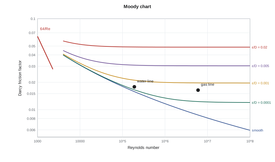
Typical absolute roughness values are about 0.046 mm (0.0018 in) for new commercial steel, rising with age, corrosion and scale. Plastic and composite lines, increasingly used for low-pressure gathering and water service, are much smoother. Internal coatings and corrosion products both change roughness, so a line's friction factor can drift over its life.

Minor losses and equivalent length

Valves, tees, bends and entrances add losses that are usually written as a loss coefficient K times the velocity head, or as an equivalent length of straight pipe. In a long gathering line these minor losses are small compared with the straight-pipe friction, but in station piping, meter runs and short flowlines they can be a large part of the total. A quick allowance of a few percent of the line length is common at the screening stage.

Gas pipeline equations

For long gas lines the density changes greatly along the line, so the pressure gradient equation is integrated with the real gas law. If temperature and the compressibility factor are taken as constant averages and the kinetic energy term is neglected, the result for a horizontal line relates flow to the difference of the squares of the inlet and outlet pressures. Several forms of this result are in use, differing in how they represent the friction factor. The Weymouth equation, published in 1912, assumes a friction factor that depends only on diameter and is widely used for small-diameter gathering lines:

In field units, q_sc is in standard cubic feet per day, temperatures in degrees Rankine, pressures in psia, L in miles and d in inches. The Panhandle equations use friction factors that depend weakly on Reynolds number and suit larger, longer transmission lines. All of these equations are special cases of the general flow equation with the Colebrook friction factor, and modern software usually solves that general form directly in segments.

# Single-phase review: Colebrook friction factor and the Weymouth gas equation
import math
SI = False  
def colebrook(Re, eD):
    if Re < 2300: return 64.0 / Re
    f = 0.02
    for _ in range(50):
        f = (-2.0 * math.log10(eD / 3.7 + 2.51 / (Re * math.sqrt(f)))) ** -2
    return f
def swamee_jain(Re, eD):
    return 0.25 / math.log10(eD / 3.7 + 5.74 / Re ** 0.9) ** 2
# liquid line: 6-inch (ID 154 mm) steel, emulsion of oil and water
D, eps = 0.154, 4.6e-5          # m
rho, mu = 900.0, 0.004          # kg/m3, Pa.s
for q_m3d in (300.0, 600.0, 900.0):
    q = q_m3d / 86400
    v = q / (math.pi * D * D / 4)
    Re = rho * v * D / mu
    f = colebrook(Re, eps / D)
    dpdl = f * rho * v * v / (2 * D)          # Pa/m
    if SI: print(f"{q_m3d:5.0f} m3/d: v = {v:4.2f} m/s, Re = {Re:7.0f}, f = {f:.4f} (Swamee-Jain {swamee_jain(Re, eps / D):.4f}), friction {dpdl * 1000 / 1000:5.0f} kPa/km")
    else:  print(f"{q_m3d * 6.2898:5.0f} bbl/d: v = {v * 3.2808:4.1f} ft/s, Re = {Re:7.0f}, f = {f:.4f} (Swamee-Jain {swamee_jain(Re, eps / D):.4f}), friction {dpdl * 0.145038 * 1.609:5.1f} psi/mile")
# Weymouth gas equation (field units), 4-inch line ID 4.026 in, 3.0 miles
Tb, pb = 520.0, 14.73          # degR, psia
T, z, SG = 520.0, 0.92, 0.70
d, Lmi = 4.026, 3.0
for p1, p2 in ((900.0, 800.0), (900.0, 700.0)):
    q_scfd = 433.5 * (Tb / pb) * math.sqrt((p1 * p1 - p2 * p2) / (SG * T * Lmi * z)) * d ** 2.667
    if SI: print(f"Weymouth: {p1 * 6.895:5.0f} -> {p2 * 6.895:5.0f} kPa(a) over {Lmi * 1.609:.1f} km gives {q_scfd * 0.0283168 / 1000:6.1f} thousand m3/d")
    else:  print(f"Weymouth: {p1:4.0f} -> {p2:4.0f} psia over {Lmi:.1f} miles gives {q_scfd / 1e6:5.2f} MMscf/d")

 1887 bbl/d: v =  0.6 ft/s, Re =    6459, f = 0.0352 (Swamee-Jain 0.0355), friction   0.8 psi/mile
 3774 bbl/d: v =  1.2 ft/s, Re =   12918, f = 0.0294 (Swamee-Jain 0.0295), friction   2.8 psi/mile
 5661 bbl/d: v =  1.8 ft/s, Re =   19378, f = 0.0267 (Swamee-Jain 0.0267), friction   5.7 psi/mile
Weymouth:  900 ->  800 psia over 3.0 miles gives  8.17 MMscf/d
Weymouth:  900 ->  700 psia over 3.0 miles gives 11.21 MMscf/d

Ethan's results show the water line in turbulent flow at all three rates, with Reynolds numbers from about 6,500 to 19,000 and friction losses of 0.8 to 5.7 psi per mile. The Swamee-Jain values agree with Colebrook to better than one percent. The gas line, 3 miles long, carries about 8.2 MMscf/d for a 100 psi pressure drop, and about 11.2 MMscf/d if the outlet pressure is lowered by another 100 psi. 'Note that the gas rate does not double when the pressure drop doubles,' Sofia says. 'It goes with the difference of the squares, so you gain less each time you pull the outlet down.'

Temperature along a line

Temperature matters in pipeline design because it controls viscosity, gas density, hydrate and wax formation, and the thermal stresses in the pipe. For a buried line in steady flow, the fluid temperature approaches the ground temperature exponentially with distance. The rate of approach depends on the overall heat transfer coefficient between fluid and ground, the pipe diameter and the mass flow rate. High-rate lines stay warm for many kilometers; low-rate lines cool to ground temperature quickly. Gas lines also cool by expansion, the Joule-Thomson effect, which can drop the temperature by several degrees across a choke or along a line with a large pressure drop. Lesson 10 uses these ideas to find where wax and hydrates may form.

Single-phase checks in a multiphase design

Single-phase calculations are not just a warm-up. They give limits that bracket the multiphase answer. If all of the flow were liquid, the friction loss would be one value; if all of it were gas at the same mass rate, it would be another. The true multiphase loss usually lies between, and well above the all-liquid value in slug flow. Single-phase calculations are also used directly for water injection lines, produced-water disposal lines, fuel gas and sales gas lines, and for checking the gas or liquid outlet lines from separators.

Non-Newtonian and waxy liquids

Many crude oils, emulsions and drilling or completion fluids do not have a single viscosity. Their apparent viscosity changes with shear rate, and waxy crudes below their pour point can develop a yield stress that must be overcome before they flow at all. For these fluids the simple Reynolds number and friction factor are replaced by generalized forms based on rheological models such as the power-law or Bingham plastic model, the same models used for drilling muds. In gathering systems the effect matters most in cold weather, after shut-ins, and in heavy oil or high-water-cut lines where tight emulsions form. A line that flows easily in summer can need much more pressure to restart after a winter shutdown, a problem lesson 10 returns to.

Checking calculations against the field

Whatever method is used, the engineer should compare predicted and measured pressure drops on existing lines before trusting the method for a new one. Gathering systems usually have pressure gauges at wellheads, headers and the facility inlet, and many have transmitters that record continuously. A short exercise, collecting a week of rates and pressures and comparing them with the model, shows whether the assumed roughness, fluid properties and elevations are reasonable. Sofia keeps a spreadsheet of exactly this kind for every line in the Tamarack Lake field. 'If the model is off by thirty percent on a line we already have,' she tells Ethan, 'it will be off by at least that much on the one we have not built yet.'

Discrepancies usually have simple causes: an elevation profile taken from an old map, a partly closed valve, wax or scale deposits that reduce the inside diameter, or gas and liquid rates allocated from a test separator that is out of calibration. Finding and fixing these problems is often worth more than choosing a better correlation.