
PET-260 · Lesson 12 of 12 · 19 min
EOS characterization, tuning and applications
Prairie Crest's management has two questions for the reservoir team. Can carbon dioxide from a nearby capture project be injected into the main Tamarack Lake oil pool to recover more oil and store the CO₂? And should the deep condensate be produced by depletion or by cycling dry gas back into it? Both answers depend on a fluid model that can predict how the reservoir fluids behave with gases that are not in them today. Nadia gives Ethan the full PVT data set, including a slim-tube test run at a commercial core laboratory in Denver, and asks him to build and tune that model with her.
The heavy-fraction problem
An equation of state needs critical properties and acentric factors for every component. For methane through the hexanes, these are known exactly. But the heptanes-plus fraction of a reservoir oil contains thousands of different molecules, from paraffins to aromatics to asphaltenes, and their individual properties are unknown. Laboratories report C₇+ as a single fraction with a measured molar mass and specific gravity, or, with gas chromatography, as single carbon number fractions up to C₂₀+, C₃₀+ or C₃₆+. Turning this information into a small set of pseudo-components with assigned properties is called characterization, and it controls the quality of every EOS prediction for oils and condensates.
Splitting the plus fraction
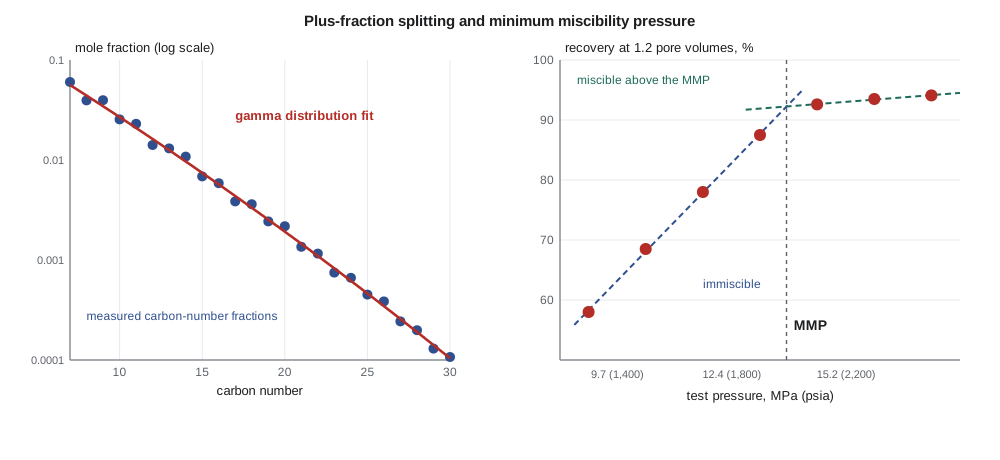
The first step is to describe how the mole fraction of the plus fraction is distributed over carbon numbers or molar mass. Katz proposed an exponential decline of mole fraction with carbon number for condensates. Whitson's three-parameter gamma distribution is more flexible and is widely used for both oils and condensates: it fits the measured single carbon number data, or, if only the plus fraction is known, distributes it with a default shape. The molar mass and specific gravity of each carbon number fraction come from the generalized tables of Katz and Firoozabadi, or from correlations based on the Watson characterization factor, which is constant for a given oil family and links boiling point to specific gravity.
Here Tb is the normal boiling point in degrees Rankine and γ the specific gravity. Paraffinic fractions have Kw of about 12.5 to 13, naphthenic fractions about 11 to 12, and aromatic fractions about 10 to 11. The value of Kw is the most useful single number for describing the chemistry of a heavy fraction.
Critical properties of pseudo-components
Each fraction then needs a critical temperature, critical pressure and acentric factor. These come from correlations in terms of boiling point and specific gravity, such as those of Kesler and Lee, Riazi and Daubert, or Twu. Different correlations give noticeably different values, and the choice affects the predicted saturation pressures by several percent. There is no right answer; engineers choose a consistent set and tune it. Finally, the many carbon number fractions are lumped into a few pseudo-components, often three to five, to keep the simulation fast. A common modern characterization uses about eight to twelve components: N₂, CO₂, C₁, C₂, C₃, lumped C₄ to C₆, and three or four heavy pseudo-components.
Tuning the EOS
An untuned EOS with a reasonable characterization usually predicts saturation pressures within about 5 to 15 percent and liquid densities, without volume translation, within 5 to 15 percent. That is not good enough for reservoir engineering. The model is tuned, or regressed, by adjusting a small number of uncertain parameters until it matches the laboratory data. Good practice adjusts only parameters that are genuinely uncertain: the critical properties and acentric factors of the heavy pseudo-components, the binary interaction parameters between methane and the heavy pseudo-components, and the volume shift parameters. The properties of the well-defined light components are left alone.
The data used in tuning should cover the processes the model will simulate. For depletion, that means the saturation pressure, CCE relative volumes, DL or CVD data, and separator test results. For gas injection, it must also include tests with the injection gas: swelling tests, which measure the saturation pressure and swelling factor as injection gas is added to the oil, and multiple-contact or slim-tube tests. A model tuned only to depletion data may predict depletion well and gas injection badly. The tuned model should then be checked against data not used in the regression, and its parameters should remain physically reasonable: critical temperatures that rise with molar mass, and acentric factors between 0 and about 1.5.
| Data | What it constrains | Typical tuning parameters |
|---|---|---|
| Saturation pressure | Phase boundary at reservoir temperature | kᵢⱼ between C₁ and heavy pseudo-components, heavy Tc and pc |
| CCE and CVD volumes, liquid dropout | Phase split and volumes below saturation | Heavy acentric factors, characterization shape |
| Liquid and stock-tank densities | Volumes and formation volume factors | Volume shift parameters |
| Separator tests | Surface yields, GOR and API | Lumping scheme, intermediate kᵢⱼ |
| Swelling and slim-tube tests | Behavior with injection gas | kᵢⱼ between injection gas components and heavy fractions |
Compositional grading
In thick reservoirs, gravity causes heavy components to concentrate at the bottom and light components at the top, even with no flow. Near-critical fluids are most affected: a reservoir can contain gas condensate at the top, volatile oil at the bottom, and a gas-oil contact where the fluid passes through its critical point without a sharp interface. An EOS model with the isothermal gravity equilibrium calculation predicts these gradients from a single sample at a reference depth. Samples from several depths test the prediction, and help locate the gas-oil contact in an appraisal well that does not penetrate it.
Gas cycling in condensate reservoirs
Lesson 9 showed that depletion leaves most of the retrograde liquid in the reservoir. Gas cycling re-injects dry gas, stripped of its liquids at a gas plant, to keep reservoir pressure above the dew point while the rich gas is produced. The liquids are sold, and the dry gas is produced at the end of the project. Cycling recovers much more condensate but delays gas sales, so its value depends on the condensate yield, the gas price and the sweep efficiency of the injected gas. The tuned EOS predicts the liquid yields for both cases, and a compositional simulation compares them. For the deep Tamarack Lake condensate, the model predicts that cycling increases condensate recovery from about 35 percent to about 60 percent of the initial condensate in place, a result Nadia will test with an economic model.
Miscible gas injection and the MMP
When a gas such as CO₂ or a rich hydrocarbon gas contacts reservoir oil at high enough pressure, the two can develop miscibility: components transfer between them until no interface remains, and the oil is displaced almost completely from the pores the gas sweeps. The minimum miscibility pressure (MMP) is the lowest pressure at which this happens at reservoir temperature. CO₂ develops miscibility mainly by extracting intermediate components, C₅ to C₃₀, from the oil, a vaporizing mechanism; rich hydrocarbon gases do it mainly by giving intermediates to the oil, a condensing mechanism, often combined with vaporizing in practice.
The slim-tube test is the standard laboratory measurement. A long, narrow tube packed with sand or glass beads is saturated with reservoir oil and flooded with gas at constant pressure and reservoir temperature. The oil recovery after 1.2 pore volumes of gas injection is plotted against test pressure. Recovery rises steeply with pressure while the displacement is immiscible, then levels off once it becomes miscible; the break-over point is taken as the MMP. Correlations such as Yellig and Metcalfe's for CO₂, which depends only on temperature, give a first estimate. A tuned EOS can calculate MMP with the method of characteristics or with multiple-mixing-cell calculations.
The Yellig-Metcalfe correlation gives MMP in psia with T in °F, and is valid for pure CO₂ and temperatures of about 95 to 192 °F (35 to 89 °C). Its constants here are as commonly published and should be treated as approximate. Impurities change the MMP: nitrogen and methane in the CO₂ raise it, and hydrogen sulfide and ethane lower it.
# Slim-tube minimum miscibility pressure from recovery data, compared with a CO2 MMP correlation
SI = False
tube = [(1300, 58.0), (1500, 68.5), (1700, 78.0), (1900, 87.5), (2100, 92.6), (2300, 93.5), (2500, 94.1)]
# fit straight lines to the steep (immiscible) and flat (miscible) parts and intersect them
def fit(pts):
    n = len(pts); sx = sum(p for p, _ in pts); sy = sum(r for _, r in pts)
    sxx = sum(p * p for p, _ in pts); sxy = sum(p * r for p, r in pts)
    m = (n * sxy - sx * sy) / (n * sxx - sx * sx); return m, (sy - m * sx) / n
m1, b1 = fit(tube[:4]); m2, b2 = fit(tube[4:])
mmp = (b2 - b1) / (m1 - m2)
print(f"slim-tube recovery at 1.2 pore volumes injected; break-over at {mmp:,.0f} psia" +
      (f" ({mmp * 6.895 / 1000:.1f} MPa)" if SI else ""))

T = 140.0                                     # reservoir temperature, F
mmp_ym = 1833.7217 + 2.2518055 * T + 0.01800674 * T**2 - 103949.93 / T   # Yellig-Metcalfe (approximate)
print(f"Yellig-Metcalfe CO2 MMP estimate at {T:.0f} F: {mmp_ym:,.0f} psia")
p_res = 2900.0                                # current average reservoir pressure, psia
for name, v in (('slim tube', mmp), ('correlation', mmp_ym)):
    margin = p_res - v
    state = "miscible" if margin > 0 else "below MMP (near-miscible or immiscible)"
print(f" {name}: reservoir pressure margin {margin:+,.0f} psi -> {state}")slim-tube recovery at 1.2 pore volumes injected; break-over at 1,993 psia Yellig-Metcalfe CO2 MMP estimate at 140 F: 1,759 psia slim tube: reservoir pressure margin +907 psi -> miscible correlation: reservoir pressure margin +1,141 psi -> miscible
The slim-tube data give an MMP of about 1,993 psia, and Yellig-Metcalfe gives 1,759 psia at 140 °F. With average reservoir pressure of 2,900 psia, the main Tamarack Lake pool is comfortably above both estimates, so CO₂ injection should be miscible if pressure is maintained. Ethan notes that the correlation is about 12 percent below the measurement, a reminder that correlations give a starting point and that the slim-tube result, matched by the tuned EOS, should drive the design.
Worked problem
MMP from a correlation
Estimate the CO₂ MMP for a reservoir at 140 °F with the Yellig-Metcalfe correlation, and compare it with a reservoir pressure of 2,900 psia.
Show solution
- MMP = 1,833.72 + 2.2518 × 140 + 0.01801 × 140² − 103,950/140.
- = 1,833.72 + 315.25 + 352.98 − 742.50 = 1,759 psia.
- Margin = 2,900 − 1,759 = 1,141 psi above the MMP.
Answer: A comfortable margin above the MMP allows for pressure falling near producers and for impurities in the CO₂ stream.
CO₂ storage and phase behavior
Injecting CO₂ for enhanced oil recovery also stores it, and carbon capture and storage projects in saline aquifers and depleted fields rely on the same phase behavior. Pure CO₂ has a critical point at 31.0 °C (87.9 °F) and 7.38 MPa (1,070 psia). At typical storage depths below about 800 m (2,600 ft), it is a dense supercritical fluid with a density of 600 to 800 kg/m³ (37 to 50 lb/ft³), so a given mass occupies much less pore volume than it would as a gas. CO₂ dissolves in brine, a few percent by mass at reservoir conditions, and the CO₂-saturated brine is slightly denser than the original brine, so it sinks; this solubility trapping, together with residual trapping and slow mineralization, makes storage more secure over time. Impurities in captured CO₂, such as nitrogen, oxygen, argon and hydrogen, change the phase envelope and density, and must be included in the EOS model for pipelines and wells.
PET-200 Introduction to Petroleum Engineering introduced CCS within the energy transition. In North Dakota, the state holds primacy for Class VI CO₂ storage wells, and the Williston Basin has active CO₂ storage and EOR projects. Phase behavior links these projects to the reservoir engineering of this course: the same EOS, tuned with the same care, predicts injectivity, plume density and the pressure response of the storage formation.
Bringing the course together
Every topic in this course feeds the fluid model. Chemistry and molar mass come from Lesson 1, phase envelopes and fluid types from Lessons 2 and 3. Gas, oil and water properties and their correlations, from Lessons 4 to 6, provide quick estimates and checks. Sampling and laboratory experiments, from Lessons 7 to 9, provide the data. Flash calculations and equations of state, from Lessons 10 and 11, provide the engine. Characterization and tuning, in this lesson, turn the engine into a model that predicts the reservoir. The reservoir simulation and enhanced recovery courses that follow will use that model as a given; knowing how it was built is what allows an engineer to question it.
Common mistakes
MistakeTuning light-component critical properties to match data.
InsteadAdjust only uncertain parameters: heavy pseudo-components, their kᵢⱼ and volume shifts.
MistakeTuning to depletion data and using the model for gas injection.
InsteadInclude swelling and slim-tube or multiple-contact data in the regression.
MistakeRelying on an MMP correlation alone to design a CO₂ flood.
InsteadMeasure the MMP with a slim-tube test and match it with the tuned EOS.
MistakeIgnoring impurities in captured CO₂.
InsteadInclude nitrogen, oxygen and other impurities in the EOS for MMP, density and pipeline design.
Summary and key terms
- Characterization splits the plus fraction, assigns critical properties and lumps pseudo-components.
- EOS tuning adjusts only uncertain parameters to match saturation pressures, volumes, densities and injection tests.
- Compositional grading and gas cycling are predicted with tuned EOS models.
- The MMP is measured by slim-tube tests and estimated by correlations such as Yellig-Metcalfe.
- CO₂ storage relies on the dense supercritical phase and on solubility, residual and mineral trapping.
- Characterization
- Describing the plus fraction as pseudo-components with assigned EOS properties.
- Watson characterization factor
- The ratio of the cube root of boiling point to specific gravity, indicating oil chemistry.
- Lumping
- Combining many components into fewer pseudo-components.
- Swelling test
- A test that measures the saturation pressure and volume of oil as gas is added.
- Minimum miscibility pressure
- The lowest pressure at which injected gas and oil develop miscibility at reservoir temperature.
- Gas cycling
- Re-injecting dry gas into a condensate reservoir to keep pressure above the dew point.
Practice problems
Work each problem on paper first, then reveal the answer to check.
A fraction has Tb = 900 °R and γ = 0.78. Find Kw.
Show answer
900^(1/3) = 9.655; Kw = 9.655/0.78 = 12.4, a mostly paraffinic fraction.
Why are light-component critical properties not tuned?
Show answer
They are known accurately; changing them would hide errors in the heavy fraction.
Slim-tube recovery levels off above 2,000 psia. What does this indicate?
Show answer
The MMP is near 2,000 psia; above it the displacement is miscible.
Why is supercritical CO₂ preferred for storage at depth?
Show answer
Its high density stores more mass in the available pore volume.
Lesson quiz · 5 questions
Score 60% or more to complete this lesson.
Create a free account to save your progress, take quizzes and earn a certificate.