
NUC-410 · Lesson 3 of 12 · 21 min
Deterministic safety analysis
Hana's first real task is to review one chapter of the safety analysis report: the large-break loss-of-coolant accident. Dr. Rohan Desai, whom she worked with in thermal hydraulics, comes over to help. "You know the physics," he says. "What is new here is the discipline. Every assumption has to be written down and justified, every code has to be qualified for the job, and every result has to be compared with an acceptance criterion. The reviewer at the NRC will read this chapter looking for the one assumption that is not conservative."
What deterministic analysis does
Deterministic safety analysis takes a specified event, such as a pipe break or a loss of feedwater, and calculates how the plant responds over time, using models of the reactor physics, thermal hydraulics, fuel behavior and containment. It then compares the calculated results with acceptance criteria: limits on fuel temperature, cladding temperature and oxidation, pressure, and radiation dose. The analysis is called deterministic because it asks a yes-or-no question about a defined scenario: given this event and these assumptions, are the criteria met? It does not ask how likely the scenario is; that is the role of probabilistic analysis.
Deterministic analysis is the backbone of licensing. It shows that each design basis event is handled by the safety systems within limits, it sets the operating limits and conditions that keep the plant inside the analyzed envelope, and it defines the set points for trips and safety system actuation. When a plant changes its equipment or its operating limits, the deterministic analysis is redone or confirmed to show that the margins remain. The analysis also feeds emergency procedures, operator training and the design of simulators.
Acceptance criteria
Acceptance criteria translate the safety functions into numbers that can be calculated. They come in two kinds. Derived criteria are limits on physical quantities that ensure a barrier stays intact, such as a peak cladding temperature or a fuel enthalpy. Dose criteria limit the radiological consequences to the public. Derived criteria are usually set with margin below the physical failure point, so that meeting them gives confidence that the barrier really holds.
| Event class | Typical derived criteria | Dose criterion |
|---|---|---|
| Moderate-frequency incident | no fuel failure; minimum departure from nucleate boiling ratio above limit; pressure below 110 percent of design | small fraction of 10 CFR 50.67 limits |
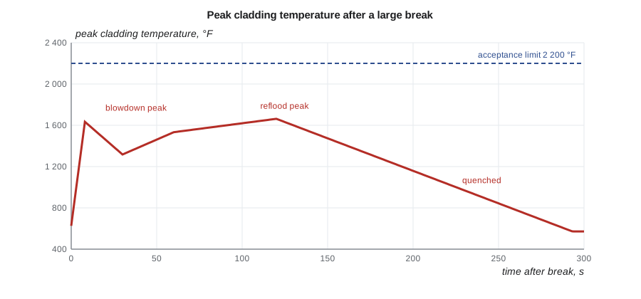
| Limiting fault, loss of coolant | peak cladding temperature below 1 204 °C (2 200 °F); local oxidation below 17 percent; hydrogen below 1 percent of cladding reacted; coolable geometry; long-term cooling | within 10 CFR 50.67 limits |
| Reactivity-initiated accident | fuel enthalpy limits; coolable geometry | within 10 CFR 50.67 limits |
For light water reactors, 10 CFR 50.46 sets five criteria for the emergency core cooling system: peak cladding temperature not above 1 204 °C (2 200 °F), maximum local oxidation not above 17 percent of cladding thickness, core-wide hydrogen generation not above 1 percent of the cladding that could react, a coolable core geometry, and long-term cooling. The criteria date from the ECCS rulemaking hearings of the early 1970s.
Codes and models
The calculations use system codes that solve the conservation equations for mass, momentum and energy in a network of volumes and junctions representing the reactor coolant system, together with models for heat transfer, two-phase flow, critical flow at the break, pumps, valves and control systems. They are coupled to reactor kinetics models, fuel and cladding models, and containment codes. Each code must be qualified: its models must be validated against separate-effects experiments, which test one phenomenon at a time, and integral experiments, which test the whole system in a scaled facility.
US system codes include TRACE, developed by the NRC, and RELAP5, along with vendor codes. Validation draws on facilities such as LOFT, Semiscale and many separate-effects tests. The NRC's evaluation model rules require that the code and its application be documented and reviewed, and Regulatory Guide 1.203 describes how evaluation models are developed and assessed.
Conservative and best-estimate approaches
There are two broad approaches to deterministic analysis. The conservative approach uses conservative models, conservative initial and boundary conditions and the worst single failure, so that the calculated result is pessimistic by construction. It is simple to review but can greatly overstate the consequences, which can lead to unnecessary operating restrictions. The best-estimate approach uses realistic models and data, then quantifies the uncertainty in the result, so that the analyst can state, with high confidence, that the true value lies below a given bound.
A common best-estimate method samples the uncertain inputs, such as gap conductance, break discharge coefficient, decay heat and heat transfer coefficients, from their probability distributions, runs the code many times and takes a high percentile of the results. With Wilks' formula, 59 random runs are enough to state with 95 percent confidence that the largest result bounds the 95th percentile of the true distribution. The best-estimate plus uncertainty approach is now widely used for loss-of-coolant analysis in both countries, alongside conservative analysis for many other events.
In the equation, γ is the percentile to be bounded (0.95) and β the confidence level (0.95). The result, 59 runs, is the smallest sample in which the highest calculated value is a 95/95 bound. Using the second-highest value requires more runs, about 93, and gives a tighter estimate.
A simple heat-up estimate
Before reading a code output, a good analyst makes a hand estimate. For a fuel rod with no cooling at all, the decay heat goes into raising the temperature of the fuel and cladding. The program below uses the Way–Wigner decay heat approximation and treats each rod as a single lump. The answer is crude but instructive: it shows how quickly the fuel heats up if emergency cooling is late, and why the timing of emergency core cooling matters so much.
# Lumped heat-up of a fuel rod after cooling is lost (illustrative, not a licensing method).
# Decay heat follows the Way-Wigner approximation; the rod is a single lump
# that heats adiabatically until cooling is restored.
P0 = 3411e6          # W thermal, full power before shutdown
T_op = 1.0e7         # s of operation before shutdown (about 4 months)
def decay(t):
    return 0.0622 * P0 * (t ** -0.2 - (t + T_op) ** -0.2)
rods = 50952          # number of fuel rods in the core
m_rod, cp = 3.0, 330.0  # kg of fuel and cladding per rod, J/(kg K)
T = 600.0             # K at the start of heat-up
t, dt = 30.0, 1.0
while T < 1477.0:
    q = decay(t) / rods          # W per rod
    T += q * dt / (m_rod * cp)
    t += dt
    if int(t) % 120 == 0:
        print(f"t = {t:4.0f} s  decay heat {decay(t)/1e6:6.1f} MW  rod temperature {T-273:6.0f} C")
print(f"with no cooling at all the rod reaches 1 204 C after about {t/60:.0f} minutes")
print("emergency core cooling must restore water well before then")t = 120 s decay heat 73.0 MW rod temperature 474 C t = 240 s decay heat 62.5 MW rod temperature 634 C t = 360 s decay heat 56.9 MW rod temperature 775 C t = 480 s decay heat 53.3 MW rod temperature 906 C t = 600 s decay heat 50.6 MW rod temperature 1030 C t = 720 s decay heat 48.5 MW rod temperature 1148 C with no cooling at all the rod reaches 1 204 C after about 13 minutes emergency core cooling must restore water well before then
The adiabatic estimate gives about thirteen minutes to reach the cladding temperature limit with no cooling at all. Real codes show faster heat-up in the hottest rods because of the power peaking and the stored energy released early in the blowdown, and slower heat-up where steam cooling continues. The estimate tells the analyst the order of magnitude of the time available, which is the kind of check that catches input errors in a code run.
Worked problem
Wilks sample size
How many code runs are needed to show, with 95 percent confidence, that the largest result bounds the 99th percentile?
Show solution
- Use n ≥ ln(1 − β)/ln γ with β = 0.95 and γ = 0.99.
- ln 0.05 = −2.996; ln 0.99 = −0.01005.
- n ≥ 2.996/0.01005 ≈ 298.
Answer: About 298 runs are needed, five times more than for the 95th percentile.
Documentation and review
A deterministic safety analysis is only as good as its documentation. For each event the report states the event description and frequency category, the acceptance criteria, the code and models used and their qualification, the plant model and its nodalization, the initial and boundary conditions with their justification, the single failure assumed, the operator actions credited and their timing, the results, the comparison with criteria, and sensitivity studies on the key parameters. An independent reviewer within the licensee checks the analysis before the regulator sees it.
Regulators review the analysis with their own experts and often run their own calculations with independent codes. Disagreements usually concern assumptions: whether an initial condition is truly limiting, whether a model is valid outside its tested range, or whether an operator action can be completed in the time assumed. Over decades, this process has produced large bodies of qualified methods and has also exposed real issues, such as the effects of fuel burnup on cladding behavior and the effect of debris on sump strainers, which led to plant modifications.
The NRC's Standard Review Plan, NUREG-0800, Chapter 15, describes how the staff review each class of transient and accident in a safety analysis report, and Regulatory Guide 1.157 and later guidance describe acceptable best-estimate methods for loss-of-coolant analysis.
Conservative and best-estimate approaches
Deterministic analysis can be carried out in several ways. In a fully conservative analysis, the computer code itself contains conservative models, and the inputs, such as initial power, decay heat and the availability of systems, are set at unfavorable values. This approach is simple to apply and to review, but the combined conservatism is unknown and can be so large that it hides real margins or distorts the order of importance of phenomena. In a best-estimate analysis, the code models the physics as realistically as possible, and the uncertainty in the result is quantified, either by statistical sampling of uncertain inputs and models or by bounding calculations. Many regulators now accept best-estimate plus uncertainty methods for the most demanding accidents, such as large break loss-of-coolant accidents.
Between the two lies a mixed approach in which a best-estimate code is used with conservative inputs for the parameters that matter most. Whichever approach is used, the analysis must show that the acceptance criteria are met with margin, that the important phenomena are modeled, and that the code has been validated against experiments that cover the relevant conditions. Validation matrices compiled by international groups list the separate-effects and integral tests that a code for a given reactor type and accident should reproduce.
Assumptions about systems and operators
Deterministic analysis also makes conservative assumptions about how systems and people behave. Non-safety systems that might help, such as the normal control systems, are usually assumed to fail or to act in the most unfavorable way. The single failure criterion requires that the safety function be achieved even if the most limiting single active component fails, in addition to the initiating event. Offsite power is often assumed to be lost at the time of the accident. Operator actions are credited only after a minimum time, commonly fifteen to thirty minutes for actions in the control room, so that the plant must protect itself automatically in the early part of the transient.
These assumptions make the analysis demanding, and they explain why plants have redundant trains, automatic actuation and diverse means of shutdown. They also explain why deterministic analysis alone cannot show which sequences are most likely, because it deliberately chooses unfavorable combinations without regard to their probability. That is the role of probabilistic assessment, which the next lessons introduce, and the two approaches are used together.
Margins and the safety case
The output of deterministic analysis is not only a list of results that meet criteria but a demonstration of margin: how far the result is from the limit and how confident the analyst is in that distance. A peak cladding temperature of 1 050 °C against a limit of 1 204 °C has a margin of about 150 degrees, but its meaning depends on the uncertainty of the calculation. Regulators look for margins that are robust, so that a reasonable change in assumptions does not lead to a limit being exceeded, and they expect licensees to track how margins change as plants age, fuel designs change and power is uprated.
Common mistakes
MistakeDeterministic analysis shows an accident cannot happen.
InsteadIt shows that, if the event happens, the plant response meets the acceptance criteria.
MistakeBest-estimate analysis is less safe because it is not conservative.
InsteadIt replaces stacked pessimism with a quantified uncertainty bound, which is often more defensible.
MistakeA validated code can be used for any event.
InsteadValidation applies to the phenomena and conditions tested; use outside that range needs justification.
Summary and key terms
- Deterministic analysis calculates the plant response to defined events and compares it with acceptance criteria.
- Acceptance criteria protect the barriers and limit public dose.
- System codes must be qualified against separate-effects and integral tests.
- Conservative analysis stacks pessimistic assumptions; best-estimate analysis quantifies uncertainty.
- Wilks' formula gives the number of runs needed for a stated percentile and confidence.
- Deterministic analysis
- Calculation of plant response to a specified event to check acceptance criteria.
- Acceptance criterion
- A limit on a calculated quantity that ensures a barrier holds or a dose limit is met.
- Best-estimate plus uncertainty
- Realistic modeling with a quantified statistical bound on the result.
- Code qualification
- Demonstrating that a computer code is valid for its intended application.
- Nodalization
- The division of the plant into volumes and junctions in a system code model.
- Wilks formula
- A statistical rule giving the sample size for a tolerance bound.
Practice problems
Work each problem on paper first, then reveal the answer to check.
Name two of the US loss-of-coolant acceptance criteria.
Show answer
Peak cladding temperature below 1 204 °C, and local oxidation below 17 percent, among others.
What is the difference between separate-effects and integral tests?
Show answer
Separate-effects tests isolate one phenomenon; integral tests reproduce the whole system response.
How many runs give a 95/95 bound using the highest value?
Show answer
59.
Why make a hand estimate before reading code results?
Show answer
To check the order of magnitude and catch input errors.
What does a deterministic analysis not tell you?
Show answer
How likely the event or its consequences are.
Lesson quiz · 5 questions
Score 60% or more to complete this lesson.
Create a free account to save your progress, take quizzes and earn a certificate.