
MSAZ-121 · Lesson 5 of 12 · 18 min
Large-scale analytics and the data warehouse
▶ Video coming soon A video version of this lesson is on the way.
Keiko's nightly sales report is a small analytics system. Every morning it pulls the previous day's transactions from StockLine, adds them to a history table, and summarizes them by store, department and week. For seven years it has worked because the data was modest and the questions were fixed. Now the questions are changing. Finance wants margins by supplier across three years. Marketing wants loyalty members' baskets compared with non-members'. Store operations wants sales beside door counts and weather. The history table has 190 million rows, and the queries that answer these questions run for an hour and slow StockLine for everyone else.
At the clinic on November 10, 2026, Nikolai drew the problem on the whiteboard. StockLine is a transactional system: it handles thousands of small reads and writes a minute, each touching a few rows, and it must stay fast for the tills. Keiko's questions are analytical: each reads millions of rows, summarizes them, and changes nothing. Running both kinds of work on the same database makes both worse. Large-scale analytics separates them.
Transactional and analytical workloads
MSAZ-120 introduced the two workload types. Online transaction processing (OLTP) systems record business events as they happen: a sale, a payment, a change of address. They are optimized for many concurrent small operations, use normalized schemas to avoid duplicated data, and enforce transactions so that each change is all-or-nothing. Online analytical processing (OLAP) systems, also called analytical workloads, answer questions about many events: totals, trends, comparisons. They are optimized for large reads, often use denormalized schemas to make queries simpler and faster, and are loaded in bulk rather than row by row.
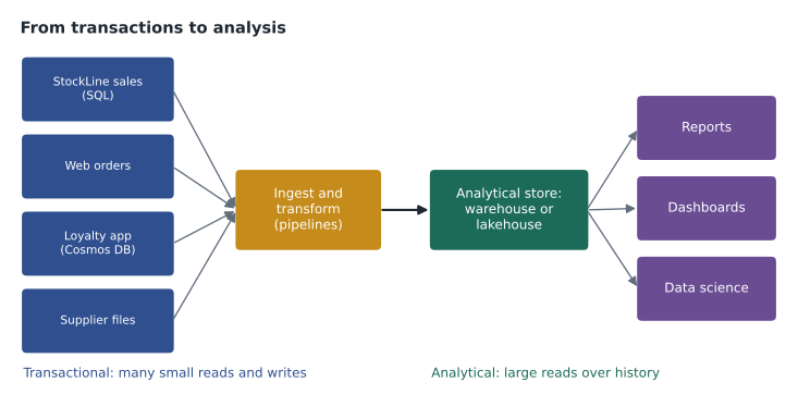
A large-scale analytics solution usually has four parts. Ingestion copies data from operational sources. Processing cleans, combines and reshapes it. An analytical data store holds the prepared data in a form that is fast to query. Analysis and visualization tools, such as Power BI, let people explore it. Lessons 5 to 8 cover these parts; lessons 11 and 12 cover visualization.
The data warehouse
A data warehouse is a relational database designed for analysis. It holds history from many sources, cleaned and integrated, in tables shaped for reporting. Users query it with SQL, and reporting tools connect to it directly. A warehouse is usually loaded on a schedule, nightly or hourly, and its data does not change once loaded except through further loads.
Warehouses usually organize data in a star schema. At the center is a fact table, which records measurable events, such as each line of each sale, with numeric measures such as quantity and amount and keys that point to dimensions. Around it are dimension tables, which describe the context of each event: the date, the store, the product, the customer. Each dimension holds descriptive attributes that people filter and group by, such as a product's department, a store's province or state, or a date's week and fiscal quarter.
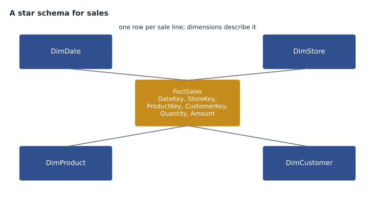
A star schema is denormalized compared with an OLTP schema. The product dimension, for example, holds the product's name, department and category in one table, even though StockLine stores categories in a separate table. That duplication is deliberate: it means most questions need only one join from the fact table to each dimension, which both people and query engines handle well. When a dimension is split into further related tables, the design is called a snowflake schema; it saves space but needs more joins.
# A tiny star schema in sqlite: one fact table, two dimensions
import sqlite3
db = sqlite3.connect(":memory:")
db.executescript("""
CREATE TABLE DimStore (StoreKey INTEGER PRIMARY KEY, StoreName TEXT, Region TEXT);
CREATE TABLE DimProduct (ProductKey INTEGER PRIMARY KEY, Product TEXT, Department TEXT);
CREATE TABLE FactSales (StoreKey INT, ProductKey INT, Qty INT, Amount REAL);
INSERT INTO DimStore VALUES (1,'Ames','West'),(2,'Store 12','East');
INSERT INTO DimProduct VALUES (1,'Patio chair','Outdoor'),(2,'Paint roller','Paint'),(3,'Grill cover','Outdoor');
INSERT INTO FactSales VALUES (1,1,4,239.96),(1,2,10,79.90),(2,1,2,119.98),(2,3,5,124.95),(1,3,1,24.99);
""")
q = """SELECT s.StoreName, p.Department, SUM(f.Amount)
       FROM FactSales f JOIN DimStore s ON f.StoreKey = s.StoreKey
                        JOIN DimProduct p ON f.ProductKey = p.ProductKey
       GROUP BY s.StoreName, p.Department ORDER BY 1, 2"""
for row in db.execute(q):
print(row)('Ames', 'Outdoor', 264.95)
('Ames', 'Paint', 79.9)
('Store 12', 'Outdoor', 244.93)What this code does
Builds a tiny star schema in an in-memory database: one fact table of sales linked to store and product dimension tables. A query joins them and totals sales by store and department. This is the layout data warehouses use to make reporting queries simple and fast.
The query shape in the script, facts joined to dimensions, filtered and grouped, is the shape of almost every report Keiko writes. In a real warehouse the fact table might have billions of rows, and the engine is built to scan and summarize them quickly.
How analytical engines go fast
Warehouse engines use several techniques that ordinary transactional databases do not emphasize. Columnar storage keeps each column's values together rather than each row's, so a query that sums Amount reads only that column, and similar values compress well. Massively parallel processing (MPP) splits data across many compute nodes, each scanning its share at the same time, then combines the results. Separation of storage and compute lets data sit in low-cost storage while compute is added for heavy queries and removed afterwards. And pre-computed aggregations store common totals so that dashboards do not recompute them every time.
| Technique | What it does | Why it helps analytics |
|---|---|---|
| Columnar storage | Stores each column's values together | Queries read only the columns they need; data compresses well |
| Massively parallel processing | Spreads work across many nodes | Large scans finish in a fraction of the time |
| Separate storage and compute | Data and processing scale independently | Pay for heavy compute only when it is used |
| Aggregations | Stores pre-computed totals | Dashboards answer common questions instantly |
Analytical data stores in Azure and Fabric
The DP-900 outline asks you to describe options for analytical data stores. They fall into two broad families. A data warehouse stores data in relational tables queried with SQL, as described above. A data lake stores files of any format in low-cost storage and is processed with engines such as Apache Spark; lesson 6 covers it, along with the lakehouse, which combines the two. In Microsoft's current platform, the warehouse is available as the Warehouse item in Microsoft Fabric, while Azure Synapse Analytics offers dedicated SQL pools for organizations that adopted it earlier. Azure Databricks provides SQL warehouses on top of a lakehouse. Lesson 8 compares these services.
Keiko asked whether she could simply copy StockLine to a second SQL Server and report from that. Nikolai said a read-only copy helps with load, and many companies start that way, but it does not change the shape of the data, combine other sources or keep years of history efficiently. A warehouse or lakehouse does all three.
Slowly changing dimensions
One analytical idea surprises people from transactional backgrounds. When a store moves from one sales region to another, what should last year's report show? In StockLine, the store's row is simply updated, and the old region is gone. In a warehouse, that would silently rewrite history: last year's West region sales would shrink. Warehouses handle this with slowly changing dimensions. The simplest approach overwrites the attribute when history does not matter. A common alternative adds a new row for the store with the new region and dates showing when each row was valid, so old facts keep pointing at the old row. DP-900 does not test the details, but Keiko recognized the problem immediately: her spreadsheets had been quietly rewriting history for years.
Who does what in analytics
MSAZ-120 described three data roles, and large-scale analytics shows how they work together. Data engineers, like Nikolai, build and run the ingestion pipelines, design the lake and warehouse structures, and make sure data arrives on time and correctly. Data analysts, like Keiko, explore the prepared data, build semantic models and reports, and work with the business to turn questions into measures and visuals. Database administrators look after the operational databases that feed the platform, such as StockLine's SQL Server, including performance, backups and security. In a small company one person may play several roles, but the responsibilities stay distinct.
Other roles appear as platforms grow. Data scientists build predictive models, such as a forecast of next week's sales for each store. Analytics engineers sit between engineers and analysts, shaping gold-layer tables and shared definitions. Data stewards own the meaning and quality of particular data, such as the product hierarchy. Keiko saw herself moving toward analytics engineering, since she already understood both the data and the questions.
Granularity: the most important design decision
Before building a fact table, the team must decide its grain: exactly what one row represents. For the sales warehouse, Nikolai and Keiko chose one row per line of each sale, the most detailed level StockLine records. A coarser grain, such as one row per store per day, would be smaller and faster but could never answer questions about individual products or baskets. A finer grain can always be summarized to a coarser one, but not the reverse. The rule of thumb is to store facts at the finest grain the business might reasonably need, and to add summary tables for speed if necessary.
The grain also decides which dimensions apply. A sale line has a date, a store, a product, a till and, for loyalty members, a customer. A store-day summary would lose the product and customer dimensions entirely. Keiko realized that her old Excel report had been built at the store-week grain, which was why it could never answer marketing's basket questions.
# The grain decides which questions can be answered
lines = [("Mon", "Ames", "Patio chair", 59.99), ("Mon", "Ames", "Grill cover", 24.99),
         ("Mon", "Store 12", "Patio chair", 59.99), ("Tue", "Ames", "Patio chair", 59.99)]
# Fine grain (sale lines) can be summarized to store-day...
summary = {}
for day, store, product, amount in lines:
    summary[(day, store)] = round(summary.get((day, store), 0) + amount, 2)
print("Store-day totals:", summary)
# ...and still answers product questions; the summary alone cannot
print("Patio chairs sold:", sum(1 for l in lines if l[2] == "Patio chair"))Store-day totals: {('Mon', 'Ames'): 84.98, ('Mon', 'Store 12'): 59.99, ('Tue', 'Ames'): 59.99}
Patio chairs sold: 3What this code does
Shows how the grain, the level of detail stored, limits the questions you can answer. Sale-line data can be summarised up to totals per store and day, and it can still answer how many patio chairs were sold. Once only the daily totals are kept, that product-level question can no longer be answered.
Analytical queries in plain words
Most analytical questions follow a pattern that Keiko learned to recognize: filter to the period and scope of interest, group by one or more dimension attributes, aggregate a measure, and compare with something, such as last year, a target or another group. "What were Outdoor department sales by store in October, compared with last October?" filters to October, groups by store, sums Amount for the Outdoor department, and compares with the same month a year earlier. Once the warehouse holds clean facts and well-described dimensions, writing such a question as SQL, or building it as a Power BI visual, becomes routine. The hard work is in the design and the loading, which is why lessons 6 and 7 matter as much as this one.
Keiko tested the idea on her own backlog. Of the twenty report requests waiting in her inbox, seventeen fitted the pattern exactly, and the other three needed data the company did not yet collect.
Worked problem
Facts or dimensions?
For the sales warehouse, classify each item as a fact table measure or a dimension attribute: (a) quantity sold; (b) product department; (c) sale amount; (d) store province or state; (e) fiscal week.
Show solution
- Quantities and amounts are numeric values recorded by each event and summed in reports, so they are measures.
- Department, province or state and fiscal week describe the context of the event and are used to filter and group, so they are dimension attributes.
Answer: Measures: (a) and (c). Dimension attributes: (b), (d) and (e).
Common mistakes
MistakeRunning large reports against the transactional database during business hours.
InsteadCopy the data into an analytical store designed for large reads.
MistakeNormalizing a warehouse exactly like the source system.
InsteadUse a star schema so most questions need one join per dimension.
MistakeUpdating dimension rows in place when history matters.
InsteadUse a slowly changing dimension approach that keeps the old version.
MistakeThinking a data warehouse is a different query language.
InsteadWarehouses are queried with SQL; their difference is design and engine.
Summary and key terms
- Transactional (OLTP) systems handle many small, concurrent changes with normalized schemas; analytical (OLAP) workloads read large volumes to answer questions about history.
- Large-scale analytics separates them with ingestion, processing, an analytical store and visualization.
- A data warehouse is a relational store for analysis, usually organized as a star schema of fact tables with measures and dimension tables with descriptive attributes.
- Columnar storage, massively parallel processing, separate storage and compute, and aggregations make large queries fast.
- Slowly changing dimensions preserve history when attributes change.
- OLTP
- Online transaction processing: systems that record business events as they happen.
- OLAP
- Online analytical processing: systems that answer questions across many events.
- Data warehouse
- A relational database designed and loaded for analysis and reporting.
- Fact table
- A table of measurable events with numeric measures and keys to dimensions.
- Dimension table
- A table of descriptive attributes used to filter and group facts.
- Star schema
- A design with one fact table joined directly to several dimension tables.
- Columnar storage
- Storing each column's values together to speed up analytical reads.
Practice problems
Work each problem on paper first, then reveal the answer to check.
In a star schema, which table holds the sale amount?
Show answer
The fact table.
Why are warehouses often denormalized?
Show answer
So that most questions need only simple joins, which are faster and easier to write.
What is massively parallel processing?
Show answer
Splitting a query across many compute nodes that work at the same time.
Lesson quiz · 5 questions
Score 60% or more to complete this lesson.
Create a free account to save your progress, take quizzes and earn a certificate.