
MEC-395 · Lesson 6 of 12 · 22 min
Data acquisition and sampling
Every reading on TL-3 ends its journey as a number in a file, produced by the data acquisition system, the DAQ: a cabinet of input modules, analog-to-digital converters, a clock and a computer. The DAQ is easy to take for granted because it is so convenient, but it makes decisions on the engineer's behalf that can quietly ruin a test. How often is each signal sampled? How finely are its values resolved? Are the channels read at the same moment or one after another? What happens to frequencies the engineer did not think about? This lesson goes through those questions with the TL-3 system, a 16-channel cabinet that Gilles Thériault assembled from a commercial chassis.
From continuous signal to numbers
A DAQ performs two separate operations on each signal. Sampling takes the value of the signal at discrete instants, usually equally spaced at the sampling rate \(f_s\). Quantization represents each sampled value by one of a finite set of numbers, determined by the analog-to-digital converter's resolution. Both throw information away, and both introduce errors of their own. The art of data acquisition is to ensure that what is thrown away does not matter for the measurement in hand.
The sampling theorem and aliasing
A sampled signal can represent frequencies only up to half the sampling rate, a limit called the Nyquist frequency. The sampling theorem states that a signal containing no frequencies above \(f_s/2\) is completely determined by its samples. A signal that does contain higher frequencies is not merely lost: it reappears, disguised, as a lower frequency. A component at frequency f sampled at \(f_s\) appears at the alias frequency
Aliasing is permanent. Once the samples have been taken, nothing in the data distinguishes an aliased 24 Hz component from a genuine one. The program shows how deceptive it can be. The 176 Hz vane-pass pulsation, sampled at 200 S/s, appears at 24 Hz, as if the pump were surging slowly. The VFD's 2 kHz switching ripple, sampled at 1,000 S/s, appears at 0 Hz, as a steady offset that looks exactly like a calibration error. Mains interference at 60 Hz sampled at 50 S/s appears at 10 Hz.
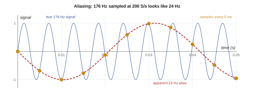
The defense is an anti-aliasing filter: an analog low-pass filter, placed before the sampler, that removes components above the Nyquist frequency before they can be sampled. Because no practical filter cuts off sharply, the sampling rate is set well above twice the highest frequency of interest, so that the filter has room to roll off. A common practice is to sample at five to ten times the highest frequency of interest with a filter cutting off a little above it. Many modern converters use delta-sigma conversion, which oversamples internally at a very high rate and applies a sharp digital filter before delivering samples at the chosen rate, giving excellent built-in protection against aliasing.
The anti-aliasing filter must be analog, or at least act before the final sampling. Averaging samples in software after they have been taken cannot remove an alias, because by then the alias is part of the data. Owen learned this when he first set up the torque channel: a software average of 1,000 S/s samples still showed a small offset that changed when the drive's carrier frequency was changed, the signature of aliased switching noise. Enabling the input module's analog filter removed it.
Choosing the sampling rate
For the steady performance test, the quantities of interest change slowly; Owen wants averages over two seconds, and nothing above about 5 Hz matters. A sampling rate of 100 S/s per channel with a 10 Hz filter is ample, and averaging 200 samples per reading reduces the remaining noise. For the pulsation measurement of Lesson 4, the frequencies of interest extend to perhaps 1 kHz, the fifth harmonic of vane pass, so Farah's test needs at least 5,000 S/s with an anti-aliasing filter around 1.2 kHz, on a channel separate from the steady-test channels. Sampling everything as fast as possible is not the answer: it fills disks, increases noise bandwidth unless filtering follows, and adds nothing to a steady measurement.
Quantization and resolution
An N-bit converter divides its input range into \(2^N\) steps. A 16-bit converter on a ±10 V range has steps of \(20/65{,}536 = 305\) µV; a 24-bit converter, 1.19 µV. Each sample is in error by up to half a step, and if the signal moves over many steps the error behaves like random noise with a rectangular distribution and rms value \(q/\sqrt{12}\), as in Lesson 3. The ideal signal-to-noise ratio of an N-bit converter for a full-scale sine wave is about \(6.02N + 1.76\) dB.
Real converters never reach their nominal resolution, because their own electronic noise exceeds the quantization step. Their performance is better described by the effective number of bits, ENOB, worked out from the measured signal-to-noise ratio. A 24-bit converter whose noise on a 10 V range is 2.4 µV rms achieves about 21 effective bits, an excellent result. The practical lesson is to compare converters by their noise specifications, not by their bit counts.
| Converter | Step on ±10 V | RMS quantization noise | Ideal SNR |
|---|---|---|---|
| 12-bit | 4.88 mV | 1.41 mV | 74 dB |
| 16-bit | 305 µV | 88 µV | 98 dB |
| 24-bit | 1.19 µV | 0.34 µV | 146 dB |
Resolution must also be judged against the signal, not the converter's range. PT-210's 4 to 20 mA signal passes through a 250 Ω precision resistor to give 1 to 5 V, which uses only a fifth of a ±10 V input range. Even so, one 16-bit step corresponds to 0.46 mbar, under 0.01 percent of the transducer's span, so quantization is negligible. A low-level signal such as a thermocouple's millivolts on the same range would be a different matter, which is why such signals are amplified first or read on a low-voltage range.
# Data acquisition on TL-3: aliasing, quantization, multiplexing and the 4-20 mA loops
import math
def alias(f, fs):
    """Apparent frequency of a sinusoid at f sampled at fs (folded into 0 .. fs/2)."""
    r = f % fs; return min(r, fs - r)
for f, fs in ((176.0, 200.0), (176.0, 1000.0), (2000.0, 1000.0), (2010.0, 1000.0), (60.0, 50.0)):
    print(f"Signal {f:6.0f} Hz sampled at {fs:6.0f} S/s appears at {alias(f, fs):6.1f} Hz")
# Quantization of an N-bit converter on a +/-10 V range
print()
for bits in (12, 16, 24):
    q = 20.0/2**bits
    print(f"{bits}-bit, +/-10 V: step {q*1e6:9.3f} uV, rms quantization noise {q/math.sqrt(12)*1e6:8.3f} uV, ideal SNR {6.02*bits + 1.76:5.1f} dB")
# A real 24-bit converter: measured noise 2.4 uV rms on the 10 V range -> effective number of bits
noise = 2.4e-6; snr = 20*math.log10((10/math.sqrt(2))/noise)
print(f"Measured noise 2.4 uV rms: SNR {snr:.1f} dB, effective number of bits {(snr - 1.76)/6.02:.1f}")
# How much of PT-210's 4-20 mA signal one 16-bit step represents through a 250 ohm resistor (1-5 V)
step_V = 20.0/2**16; step_bar = step_V/4.0*6.0
print(f"16-bit step on the 1-5 V signal of PT-210: {step_bar*1000:.2f} mbar ({100*step_bar/6:.4f} % of span)")
# Multiplexed scanning: 12 channels through one converter at 1,200 samples/s in total
ch, rate = 12, 1200.0
print(f"\n{ch} channels at {rate:.0f} S/s total: {rate/ch:.0f} S/s per channel, {1000/rate:.3f} ms between adjacent channels, scan skew {1000*(ch - 1)/rate:.2f} ms")
# 4-20 mA loop budget: supply, receiver resistor, cable, transmitter minimum voltage
Vs, Rr, Vmin = 24.0, 250.0, 10.5
Rc = 2*120*0.0175/1.0                        # 120 m of 1.0 mm2 copper, out and back, 0.0175 ohm mm2/m
Rmax = (Vs - Vmin)/0.020
print(f"Loop: cable {Rc:.1f} ohm + receiver {Rr:.0f} ohm = {Rc + Rr:.1f} ohm; maximum allowed at 20 mA {Rmax:.0f} ohm ->",
      "OK" if Rc + Rr <= Rmax else "too much")
print(f"Voltage left for the transmitter at 20 mA: {Vs - 0.020*(Rc + Rr):.1f} V (needs {Vmin} V)")
for mA in (3.2, 4.0, 12.0, 20.0, 21.5):
    state = 'fault: low' if mA < 3.6 else 'fault: high' if mA > 21.0 else 'normal'
print(f" {mA:4.1f} mA -> {(mA - 4)/16*6:6.3f} bar ({state})")Signal 176 Hz sampled at 200 S/s appears at 24.0 Hz Signal 176 Hz sampled at 1000 S/s appears at 176.0 Hz Signal 2000 Hz sampled at 1000 S/s appears at 0.0 Hz Signal 2010 Hz sampled at 1000 S/s appears at 10.0 Hz Signal 60 Hz sampled at 50 S/s appears at 10.0 Hz 12-bit, +/-10 V: step 4882.812 uV, rms quantization noise 1409.547 uV, ideal SNR 74.0 dB 16-bit, +/-10 V: step 305.176 uV, rms quantization noise 88.097 uV, ideal SNR 98.1 dB 24-bit, +/-10 V: step 1.192 uV, rms quantization noise 0.344 uV, ideal SNR 146.2 dB Measured noise 2.4 uV rms: SNR 129.4 dB, effective number of bits 21.2 16-bit step on the 1-5 V signal of PT-210: 0.46 mbar (0.0076 % of span) 12 channels at 1200 S/s total: 100 S/s per channel, 0.833 ms between adjacent channels, scan skew 9.17 ms Loop: cable 4.2 ohm + receiver 250 ohm = 254.2 ohm; maximum allowed at 20 mA 675 ohm -> OK Voltage left for the transmitter at 20 mA: 18.9 V (needs 10.5 V) 3.2 mA -> -0.300 bar (fault: low) 4.0 mA -> 0.000 bar (normal) 12.0 mA -> 3.000 bar (normal) 20.0 mA -> 6.000 bar (normal) 21.5 mA -> 6.562 bar (fault: high)
Multiplexing, skew and settling
To save cost, many DAQs use one converter shared by several channels through a multiplexer that switches between them. A 16-channel module with an aggregate rate of 1,200 S/s, scanning twelve channels, reads each channel 100 times a second, with 0.83 ms between adjacent channels and 9.2 ms between the first and last channel of a scan. For slowly varying test quantities that skew does not matter, but when two channels must be combined at the same instant, such as torque and speed to compute instantaneous power during a start-up, it can. Simultaneous-sampling DAQs give each channel its own converter or sample-and-hold, so all channels are captured at the same instant.
Multiplexers have another subtlety. After each switch, the converter's input must settle to the new channel's voltage before sampling, and a high-impedance source settles slowly. A channel can then show a small error that depends on the voltage of the channel read just before it, called crosstalk or ghosting. Buffering high-impedance sensors, slowing the scan, or adding a dummy grounded channel between sensitive ones are the usual cures.
The 4 to 20 mA current loop
Most industrial transmitters, including PT-110 and PT-210, send their signals as a current between 4 and 20 mA. Current loops have three great advantages over voltage signals. The current is the same everywhere in a series loop, so cable resistance does not affect the reading, and runs of hundreds of meters are routine. The live zero at 4 mA means that a broken wire, which gives 0 mA, is distinguishable from a true zero reading. And two-wire transmitters draw their operating power from the same loop, needing no separate supply.
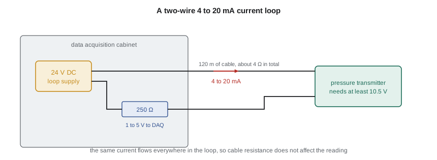
A loop works only if the supply can drive 20 mA through everything in it while leaving the transmitter its minimum operating voltage. The program checks TL-3's longest loop: 24 V supply, 250 Ω receiver, 4.2 Ω of cable, and a transmitter needing 10.5 V. The maximum total resistance at 20 mA is \((24 - 10.5)/0.020 = 675\) Ω, so the loop has ample margin. Readings below about 3.6 mA or above about 21 mA are treated as faults rather than as measurements; the program flags them, and the DAQ refuses to use them in a test result.
The receiving resistor deserves care, since the measured voltage is the current times its resistance. A 0.01 percent resistor with a low temperature coefficient contributes far less than the transmitter; an ordinary 1 percent resistor could contribute more than the transmitter's whole error. Many transmitters also superimpose a digital signal on the current using the HART protocol, which lets a technician read the transmitter's own diagnostics and its digital value through the same two wires. Fieldbus and Ethernet-based industrial networks carry fully digital measurements, avoiding conversion errors at the cost of more complex configuration.
Worked problem
Sampling a start-up record
Owen wants to record torque during a start-up, in which the torque rises and falls over about half a second, with useful detail up to 50 Hz. The drive's switching component is at 2 kHz. Choose a sampling rate and an anti-aliasing filter cutoff.
Show solution
- Highest frequency of interest: 50 Hz. Sample at about ten times that: 500 S/s, Nyquist frequency 250 Hz.
- Place the anti-aliasing cutoff a little above 50 Hz, say 80 Hz, so the band of interest is flat.
- Check the switching component: a fourth-order filter at 80 Hz attenuates 2 kHz by about \((2000/80)^4 = 3.9 \times 10^5\), or −112 dB.
Answer: Sampling at 500 S/s with a fourth-order 80 Hz filter captures the start-up transient and suppresses the drive's switching ripple far below the noise.
Records and metadata
A file of numbers is useless without knowing what they are. The TL-3 software stores, with every test, the channel list, units, scaling, calibration identities and due dates, filter settings, sampling rate, the time of every reading and the software version. Raw samples are kept alongside the averaged values, so any reading can be re-examined if a question arises. Owen insists on one more practice: no hand-entered correction is ever applied to raw data; every correction lives in documented software, so that the path from sample to certificate can be followed and repeated.
Common mistakes
MistakeAssuming averaging in software removes aliasing.
InsteadAliases must be prevented by an analog or delta-sigma filter before sampling.
MistakeSampling at exactly twice the highest frequency of interest.
InsteadSample at five to ten times, with an anti-aliasing filter just above the band.
MistakeComparing converters by bit count.
InsteadCompare noise or effective number of bits.
MistakeCombining multiplexed channels as if they were simultaneous during fast transients.
InsteadAccount for the scan skew or use simultaneous sampling.
MistakeTreating a 0 mA or 23 mA loop reading as a measurement.
InsteadValues outside about 3.6 to 21 mA indicate a fault.
Summary and key terms
- Sampling represents frequencies only up to half the sampling rate; higher ones alias to false lower frequencies.
- Aliasing is prevented by an anti-aliasing filter before sampling, not by later averaging.
- An N-bit converter has q = range/2ᴺ and rms quantization noise q/√12; real converters are judged by ENOB.
- Multiplexed DAQs read channels in sequence, with skew and settling effects; simultaneous sampling avoids them.
- 4 to 20 mA loops are immune to cable resistance and detect broken wires; the loop budget must leave the transmitter its minimum voltage.
- Every test file carries its metadata, and raw data are kept.
- Sampling rate
- The number of samples per second taken of a signal.
- Nyquist frequency
- Half the sampling rate; the highest frequency a sampled signal can represent.
- Aliasing
- The appearance of a frequency above the Nyquist frequency as a false lower frequency.
- Anti-aliasing filter
- A low-pass filter applied before sampling to remove components above the Nyquist frequency.
- Quantization
- Representing a sampled value by one of a finite set of levels.
- Effective number of bits
- A converter's resolution worked out from its measured signal-to-noise ratio.
- Multiplexer
- A switch that connects several input channels in turn to one converter.
- Scan skew
- The time difference between samples of different channels in one multiplexed scan.
- Live zero
- A signal range starting above zero, such as 4 mA, so that a failure gives an out-of-range value.
- HART
- A digital protocol superimposed on a 4 to 20 mA loop for configuration and diagnostics.
Practice problems
Work each problem on paper first, then reveal the answer to check.
A 300 Hz component is sampled at 400 S/s. At what frequency does it appear?
Show answer
|300 − 400| = 100 Hz.
What is the step size of a 16-bit converter on a ±5 V range?
Show answer
10/65,536 = 153 µV.
In the program, what is the longest cable (1.0 mm² copper, out and back) the loop could have at 20 mA?
Show answer
(675 − 250)/(2 × 0.0175) ≈ 12,100 m, far more than needed.
A converter's measured SNR is 110 dB. What is its ENOB?
Show answer
(110 − 1.76)/6.02 ≈ 18 bits.
Why is a 250 Ω receiver resistor with 1 percent tolerance unsuitable for PT-210?
Show answer
Its error alone would be 1 percent of reading, far larger than the transmitter's 0.05 percent of span.
Lesson quiz · 5 questions
Score 60% or more to complete this lesson.
Create a free account to save your progress, take quizzes and earn a certificate.