
MEC-395 · Lesson 3 of 12 · 23 min
Uncertainty analysis
The purchase order for the six TP-80 pumps guarantees 75 percent efficiency at the rated point. Suppose TL-3 measures 75.8 percent. Has the pump met its guarantee? The answer depends entirely on how well that 75.8 is known. If the uncertainty is a quarter of a percentage point, the pump has clearly passed; if it is two points, the test proves almost nothing. The pump test standards that apply to the order, ANSI/HI 14.6 and ISO 9906, recognize this by setting limits on the measurement uncertainty that a test laboratory may have, and requiring that it be evaluated. This lesson shows how Owen does that, following the international method for evaluating uncertainty.
The GUM framework
The internationally agreed method is set out in the Guide to the Expression of Uncertainty in Measurement, universally called the GUM, published by the Joint Committee for Guides in Metrology. Its approach has four steps. First, write a measurement model: an equation \(y = f(x_1, x_2, \dots, x_N)\) giving the measurand in terms of the input quantities that are actually measured or looked up. Second, evaluate a standard uncertainty \(u(x_i)\) for each input, expressed as a standard deviation. Third, combine them through the model into a combined standard uncertainty \(u_c(y)\). Fourth, multiply by a coverage factor k to obtain an expanded uncertainty U that defines an interval with a stated level of confidence, usually about 95 percent.
In North American engineering practice the same ideas appear in ASME PTC 19.1, Test Uncertainty, the uncertainty standard used with ASME's performance test codes. PTC 19.1 classifies uncertainty sources by their effect, as systematic or random, rather than by how they were evaluated, and uses its own symbols, but the arithmetic of combination is essentially the same and the two approaches give the same answers when applied consistently. Owen uses GUM terms in this lesson because the pump standards refer to them, and notes the PTC 19.1 equivalents where they help.
The measurement model for efficiency
Pump efficiency is the ratio of the power delivered to the water to the mechanical power put into the shaft:
with density ρ, gravity g, flow rate Q, total head H, speed n in rpm and shaft torque T. Head is not measured directly; it comes from its own model, built up from the discharge pressure \(p_d\) (gauge), the suction pressure \(p_s\) (absolute), the barometric pressure \(p_b\), the height difference \(\Delta z\) between the two pressure tappings, and the velocities in the suction and discharge pipes:
Writing the model down is not a formality. It shows every input that must be measured, so none is forgotten, and it shows how each enters. Here, for example, it shows that a barometer reading is needed, because the two pressure transducers on TL-3 measure on different references: PT-110 reads absolute pressure and PT-210 reads gauge pressure. Lesson 8 explains why the stand is built that way.
Type A and Type B evaluation
The GUM recognizes two ways of evaluating a standard uncertainty. A Type A evaluation uses statistics on repeated observations: the standard error of the mean from Lesson 2 is a Type A standard uncertainty. A Type B evaluation uses any other information: a calibration certificate, a manufacturer's specification, the resolution of a display, handbook values, experience. The names describe the method, not the nature of the error, and both are treated identically once evaluated. The flowmeter's random scatter at a test point is evaluated by Type A; its calibration uncertainty, taken from the weigh-tank calibration report, is Type B.
Type B information rarely arrives as a standard deviation, so it must be converted, and that requires a judgment about the shape of the distribution. If a calibration certificate states an expanded uncertainty U with coverage factor k, the standard uncertainty is U/k. If a specification says only that the error lies within ±a, with no reason to think any value in that range more likely than another, a rectangular distribution is assumed, and its standard deviation is \(a/\sqrt{3}\). If values near the center are more likely than those at the limits, a triangular distribution gives \(a/\sqrt{6}\). A digital display with resolution δ contributes a rectangular uncertainty of half-width δ/2, or \(\delta/\sqrt{12}\).
| Information available | Assumed distribution | Standard uncertainty |
|---|---|---|
| Certificate: U at coverage factor k | Normal | U/k |
| Limits ±a, any value equally likely | Rectangular | a/√3 ≈ 0.577a |
| Limits ±a, central values more likely | Triangular | a/√6 ≈ 0.408a |
| Display resolution δ | Rectangular, half-width δ/2 | δ/√12 ≈ 0.289δ |
| n repeated readings with standard deviation s | Type A | s/√n |
Sensitivity coefficients and combination
Each input's uncertainty affects the result in proportion to how strongly the result depends on that input. The sensitivity coefficient is the partial derivative \(c_i = \partial f/\partial x_i\), evaluated at the measured values. For independent inputs the combined standard uncertainty is the root sum of squares of the individual contributions:
This law of propagation of uncertainty is a first-order Taylor expansion of the model, and it is accurate when the model is close to linear over the range of the uncertainties, which is almost always true in engineering measurement. For models made only of products and quotients, like the efficiency equation, it takes a convenient relative form: the relative uncertainties add in quadrature, each multiplied by its exponent in the model. For efficiency,
Quadrature addition has a striking consequence: the largest contributions dominate completely. A contribution one third the size of the largest adds only about 5 percent to the combined uncertainty. Effort spent reducing small contributions is wasted; effort spent on the largest pays directly. An uncertainty budget, which lists every contribution and its share of the total, shows at a glance where to spend money.
If two inputs are correlated, the sum needs extra terms, \(2c_ic_j u(x_i)u(x_j)r_{ij}\), where \(r_{ij}\) is their correlation coefficient. Correlation arises when two inputs share an error source: two pressure transducers calibrated against the same deadweight tester share that tester's error, which cancels in their difference. Owen ignores such correlations in this first budget, which is conservative here, and notes them for later.
# Uncertainty budget for TP-80 efficiency at the guarantee point, by the GUM method and by Monte Carlo
import math, random
g = 9.806
def eta(Q, pd, ps, pb, dz, T, n, rho):
    """Q m3/h, pd discharge gauge bar, ps suction absolute bar, pb barometer bar, dz m, T N m, n rpm, rho kg/m3"""
    q = Q/3600; v1 = q/(math.pi*0.125**2/4); v2 = q/(math.pi*0.100**2/4)
    H = ((pd + pb) - ps)*1e5/(rho*g) + dz + (v2*v2 - v1*v1)/(2*g)
    return rho*g*q*H/(2*math.pi*n/60*T), H
# name: (value, standard uncertainty, distribution, source)
x = {'Q':   (90.08, 0.11,   'normal', 'FT-201 weigh-tank calibration 0.25 % (k = 2) plus repeatability'),
     'pd':  (3.240, 0.00173, 'rect',  'PT-210 +/-0.05 % of 6 bar span, rectangular'),
     'ps':  (1.130, 0.00115, 'rect',  'PT-110 +/-0.05 % of 4 bar span, rectangular'),
     'pb':  (1.0130, 0.00017,'rect',  'barometer +/-0.3 mbar, rectangular'),
     'dz':  (0.200, 0.0012,  'rect',  'gauge height difference +/-2 mm, rectangular'),
     'T':   (56.80, 0.0577,  'rect',  'TQ-301 +/-0.1 % of 100 N m, rectangular'),
     'n':   (1760.0, 0.577,  'rect',  'ST-301 +/-1 rpm, rectangular'),
     'rho': (998.2, 0.03,    'normal','density from TT-102 water temperature 20.0 C')}
v0 = {k: val[0] for k, val in x.items()}
e0, H0 = eta(**v0)
print(f"Head {H0:.3f} m, efficiency {100*e0:.2f} %\n")
print(" input   value      u(x_i)    sensitivity c_i   |c_i| u(x_i)   share of u_c^2")
contrib = {}
for k, (val, u, dist, src) in x.items():
    d = dict(v0); h = 1e-6*abs(val); d[k] = val + h
    c = (eta(**d)[0] - e0)/h; contrib[k] = (val, u, c, abs(c)*u)
uc = math.sqrt(sum(cu*cu for *_, cu in contrib.values()))
for k, (val, u, c, cu) in contrib.items():
    print(f"  {k:4s} {val:9.4f}  {u:9.5f}   {c:+12.5f}     {100*cu:7.4f} %pt      {100*cu*cu/uc/uc:5.1f} %")
print(f"\nCombined standard uncertainty u_c = {100*uc:.3f} percentage points ({100*uc/e0:.2f} % of reading)")
print(f"Expanded uncertainty, k = 2: efficiency = {100*e0:.2f} % +/- {200*uc:.2f} points")
# Monte Carlo propagation (JCGM 101 approach): draw every input from its distribution
random.seed(395); N = 200000; out = []
for _ in range(N):
    d = {}
    for k, (val, u, dist, src) in x.items():
        d[k] = random.gauss(val, u) if dist == 'normal' else val + random.uniform(-1, 1)*u*math.sqrt(3)
    out.append(eta(**d)[0])
out.sort(); m = sum(out)/N; s = math.sqrt(sum((v - m)**2 for v in out)/(N - 1))
lo, hi = out[int(0.025*N)], out[int(0.975*N)]
print(f"Monte Carlo, {N} trials: mean {100*m:.2f} %, standard deviation {100*s:.3f} points, 95 % interval {100*lo:.2f} to {100*hi:.2f} %")Head 32.411 m, efficiency 75.83 % input value u(x_i) sensitivity c_i |c_i| u(x_i) share of u_c^2 Q 90.0800 0.11000 +0.00858 0.0943 %pt 49.6 % pd 3.2400 0.00173 +0.23902 0.0414 %pt 9.5 % ps 1.1300 0.00115 -0.23902 0.0275 %pt 4.2 % pb 1.0130 0.00017 +0.23902 0.0041 %pt 0.1 % dz 0.2000 0.00120 +0.02340 0.0028 %pt 0.0 % T 56.8000 0.05770 -0.01335 0.0770 %pt 33.1 % n 1760.0000 0.57700 -0.00043 0.0249 %pt 3.4 % rho 998.2000 0.03000 +0.00001 0.0000 %pt 0.0 % Combined standard uncertainty u_c = 0.134 percentage points (0.18 % of reading) Expanded uncertainty, k = 2: efficiency = 75.83 % +/- 0.27 points Monte Carlo, 200000 trials: mean 75.83 %, standard deviation 0.134 points, 95 % interval 75.57 to 76.09 %
The TL-3 budget at the guarantee point
The program evaluates the full model at Owen's measured values: 90.08 m³/h, discharge pressure 3.240 bar gauge, suction pressure 1.130 bar absolute, barometer 1.0130 bar, gauge height difference 0.200 m, torque 56.80 N·m, speed 1,760 rpm and water at 20 °C. The head is 32.41 m and the efficiency 75.83 percent. Rather than differentiate by hand, the program finds each sensitivity coefficient by changing one input by a tiny amount and seeing how much the efficiency changes, a numerical approach that works for any model.
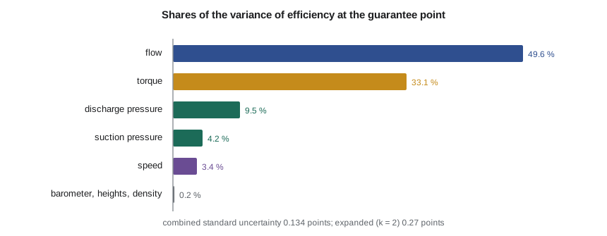
The budget is instructive. Flow contributes half of the variance and torque a third. The two pressure transducers together contribute about 14 percent, speed about 3 percent, and the barometer, height difference and density practically nothing. The density result surprises Owen until he looks at the model: density appears in the numerator of efficiency and, through the pressure term, in the denominator of head, so it cancels almost completely. The combined standard uncertainty is 0.134 percentage points, and with k = 2 the expanded uncertainty is ±0.27 points. The efficiency is 75.83 ± 0.27 percent, and the guarantee of 75 percent is clearly met.
The budget also tells Lucie where to improve the stand if a customer ever asks for tighter results. Better flow calibration would help most. The torque contribution could be cut almost in half cheaply: TQ-301's ±0.1 percent of full scale is 0.1 N·m on a 100 N·m transducer, which is 0.18 percent of the 56.8 N·m being measured. A transducer sized closer to the working torque, or one specified as a percentage of reading, would do better. Lesson 7 returns to this choice.
Coverage factors and degrees of freedom
The coverage factor k = 2 gives about 95 percent coverage when the combined uncertainty is known well, that is, when it has many effective degrees of freedom. If a Type A contribution from only a few readings dominates, k should be the Student t value for the effective degrees of freedom, found from the Welch–Satterthwaite formula:
Type B contributions are usually given very large or infinite degrees of freedom, unless there is doubt about the information itself. In the TL-3 budget the only Type A part is the flow repeatability, which is a small share of the flow contribution, and \(\nu_{\text{eff}}\) is in the hundreds, so k = 2 is appropriate.
Monte Carlo propagation
A supplement to the GUM describes a second way to propagate uncertainty that makes no linear approximation at all. Each input is drawn at random from its assumed distribution, the model is evaluated, and the process is repeated many thousands of times. The spread of the results is the uncertainty of the output, and the interval containing the central 95 percent of them is the coverage interval. Monte Carlo propagation handles strongly nonlinear models, inputs with odd distributions and outputs whose distribution is not normal, and it is easy to program. The TL-3 program runs 200,000 trials and finds a standard deviation of 0.134 points and a 95 percent interval of 75.57 to 76.09 percent, agreeing with the GUM calculation to the digits shown. For a model this close to linear the two methods must agree; the Monte Carlo result confirms that the first-order approximation is sound.
Worked problem
Uncertainty of hydraulic power
Hydraulic power is \(P_w = \rho g Q H\). At the guarantee point Q = 90.08 m³/h with standard uncertainty 0.122 percent and H = 32.41 m with standard uncertainty 0.066 percent. Density and gravity contribute negligibly. Find the expanded uncertainty of \(P_w\).
Show solution
- \(P_w = 998.2 \times 9.806 \times (90.08/3600) \times 32.41 = 7.94\) kW.
- Relative standard uncertainty: \(\sqrt{0.122^2 + 0.066^2} = 0.139\) percent.
- Expanded, k = 2: 0.28 percent, or ±0.022 kW.
Answer: \(P_w = 7.94 \pm 0.02\) kW at about 95 percent confidence. Both inputs appear to the first power, so their relative uncertainties add directly in quadrature.
Reporting uncertainty
A result is reported with its expanded uncertainty, the coverage factor and the confidence level, for example \"η = 75.8 ± 0.3 percent (k = 2, approximately 95 percent confidence)\". The uncertainty is rounded to one or two significant figures, and the result to the same decimal place. The budget itself goes in the test report or the laboratory's file, so that anyone can see how the figure was obtained. Stating an uncertainty without saying what it covers, or quoting a result to more digits than its uncertainty supports, are among the commonest faults in engineering test reports.
Common mistakes
MistakeAdding uncertainty contributions arithmetically.
InsteadIndependent contributions combine as the root sum of squares.
MistakeTreating a specification limit ±a as a standard uncertainty.
InsteadDivide by √3 for a rectangular distribution unless there is reason to choose another.
MistakeSpending effort on the smallest contributions.
InsteadReduce the largest; quadrature makes small ones nearly irrelevant.
MistakeUsing k = 2 when a few readings dominate the budget.
InsteadFind the effective degrees of freedom and use the matching Student t value.
MistakeReporting an efficiency of 75.8312 percent ± 0.27.
InsteadRound the uncertainty to one or two figures and the result to match: 75.8 ± 0.3 percent.
Summary and key terms
- The GUM method: write a model, evaluate standard uncertainties, combine them with sensitivity coefficients, expand with a coverage factor.
- Type A evaluations use statistics on repeated readings; Type B use all other information.
- Limits ±a with a rectangular distribution give a standard uncertainty of a/√3.
- Independent contributions add in quadrature, so the largest dominate.
- At the guarantee point, η = 75.83 ± 0.27 percent (k = 2); flow and torque give over 80 percent of the variance.
- Monte Carlo propagation confirms the result without any linear approximation.
- Measurement model
- The equation giving the measurand in terms of the input quantities.
- Standard uncertainty
- The uncertainty of a quantity expressed as a standard deviation.
- Type A evaluation
- Evaluation of a standard uncertainty by statistical analysis of repeated observations.
- Type B evaluation
- Evaluation of a standard uncertainty by means other than statistics on repeated observations.
- Sensitivity coefficient
- The partial derivative of the model with respect to an input, describing how the output responds to it.
- Combined standard uncertainty
- The standard uncertainty of the result, obtained by combining the input contributions.
- Coverage factor
- The multiplier applied to the combined standard uncertainty to obtain an expanded uncertainty.
- Expanded uncertainty
- A quantity defining an interval about the result expected to contain a large, stated fraction of the values that could be attributed to the measurand.
- Uncertainty budget
- A table listing each source of uncertainty, its size, sensitivity and contribution to the total.
- Monte Carlo propagation
- Propagating uncertainty by evaluating the model with inputs drawn many times from their distributions.
Practice problems
Work each problem on paper first, then reveal the answer to check.
A calibration certificate gives U = 0.4 mbar with k = 2. What is the standard uncertainty?
Show answer
0.2 mbar.
A thermometer's specification is ±0.3 °C. What standard uncertainty do you assign, assuming a rectangular distribution?
Show answer
0.3/√3 = 0.17 °C.
Three independent contributions are 0.10, 0.04 and 0.03 percent. Find the combined uncertainty.
Show answer
√(0.01 + 0.0016 + 0.0009) = 0.112 percent.
In the program, what happens to the combined uncertainty if TQ-301 is replaced by a transducer with ±0.05 percent of a 100 N·m full scale?
Show answer
The torque contribution halves to 0.039 points, and u_c falls to about 0.113 points.
Why does the uncertainty of water density hardly affect the efficiency result?
Show answer
Density multiplies hydraulic power but divides the pressure part of head, so it nearly cancels.
Lesson quiz · 5 questions
Score 60% or more to complete this lesson.
Create a free account to save your progress, take quizzes and earn a certificate.