
MEC-395 · Lesson 5 of 12 · 22 min
Signal conditioning, noise and grounding
The first time Owen opened the live display of TQ-301 with the variable-frequency drive running, the torque trace was a fuzzy band two newton-meters wide. With the drive stopped and the motor running direct on line, the band shrank to a thin line. Nothing was wrong with the torque transducer; its signal was being swamped on the way to the data acquisition system. This lesson is about that journey: how small sensor signals are converted, amplified and filtered into something worth recording, where noise comes from, and how careful wiring and grounding keep it out. Gilles Thériault, who has spent twenty years chasing electrical noise in test cells, supplies most of the practical rules.
Why conditioning is needed
Most sensors produce signals that are small, at awkward impedance levels or in the wrong form. A strain gauge changes its resistance by a tenth of a percent at full load. A thermocouple produces about 40 µV per degree. A piezoelectric accelerometer produces charge, not voltage. A data acquisition input, on the other hand, wants a voltage of a few volts, from a low-impedance source, free of noise outside the frequency band of interest. Signal conditioning bridges the gap. Its main functions are excitation (supplying the voltage or current a passive sensor needs), conversion (turning resistance, charge or current into voltage), amplification, filtering, isolation and linearization.
Bridge circuits
Resistive sensors such as strain gauges and RTDs are usually connected in a Wheatstone bridge: four resistances arranged in a diamond, with an excitation voltage across one diagonal and the output taken across the other. When all four arms are equal the bridge is balanced and the output is zero. If one arm changes by a fraction \(x = \Delta R/R\), the output is
The bridge has three great virtues. It measures a small change against a zero background rather than as a tiny change in a large voltage, so the amplifier can be set to a high gain. It compensates for effects that change all arms equally, most importantly temperature, if the arms are matched. And with more than one active arm it multiplies the signal. Two active gauges with opposite strains, as on opposite faces of a beam in bending or at ±45° on a shaft in torsion, form a half bridge with twice the output and no nonlinearity; four active gauges form a full bridge with four times the output of a quarter bridge. Lesson 7 uses exactly this arrangement for the torque transducer.
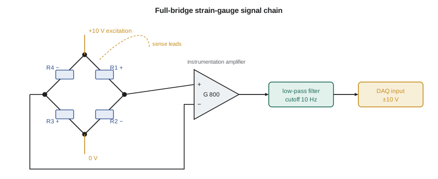
A bridge's output is proportional to its excitation, so excitation must be stable, or the measurement must be made ratiometric, dividing the output by the excitation measured at the same moment. Transducer sensitivities are therefore quoted in millivolts per volt: a load cell rated at 2.0 mV/V gives 20 mV at full load with 10 V excitation. Long cables drop some of the excitation voltage in their resistance, and that drop changes with temperature. Six-wire connections add a pair of sense leads that measure the excitation at the bridge itself, so the conditioner can regulate or ratio against it.
Amplifiers
The operational amplifier, a high-gain differential amplifier used with feedback, is the building block of nearly all conditioning circuits. With feedback resistors it forms inverting and non-inverting amplifiers whose gain is set by a resistor ratio, buffers that present a high input impedance to a sensor and a low output impedance to the next stage, integrators, active filters and many more. For bridge and thermocouple signals, the key circuit is the instrumentation amplifier, which amplifies the small difference between its two inputs while rejecting whatever voltage they have in common.
That rejection matters because a bridge's two output terminals both sit at about half the excitation voltage, 5 V, while their difference is a few millivolts. The ability to ignore the common voltage is the common-mode rejection ratio, CMRR, usually in decibels. With a CMRR of 100 dB, a common-mode voltage of 5 V produces an error equivalent to 50 µV at the input. A constant error of that kind is removed by zeroing; what matters is that common-mode voltages from interference also vary, and good instrumentation amplifiers offer 120 dB or more at the gains used for bridges, rejecting a million to one.
# Signal conditioning for a strain-gauge transducer: bridge output, amplification, filtering and noise
import math
GF, eps, Vex = 2.0, 500e-6, 10.0            # gauge factor, strain, bridge excitation (V)
x = GF*eps                                   # fractional resistance change dR/R
quarter_exact = Vex*(x/4)/(1 + x/2)          # one active gauge
quarter_lin = Vex*x/4
half = Vex*x/2                               # two active gauges, opposite strains (bending or torsion)
full = Vex*x                                 # four active gauges
print(f"dR/R = {x*1e6:.0f} parts per million for {eps*1e6:.0f} microstrain")
print(f"Quarter bridge: {quarter_exact*1000:.4f} mV (linear estimate {quarter_lin*1000:.4f} mV, nonlinearity {100*(quarter_lin - quarter_exact)/quarter_exact:.3f} %)")
print(f"Half bridge:    {half*1000:.4f} mV     Full bridge: {full*1000:.4f} mV  = {full/Vex*1000:.2f} mV/V")
# Amplify the full-bridge signal into a +/-10 V input, leaving 20 % headroom
G = 0.8*10/full
print(f"\nInstrumentation amplifier gain to put full load at 8 V: {G:.0f}")
Vcm, CMRR_dB = Vex/2, 100.0                  # bridge outputs both sit near half the excitation
err = Vcm/10**(CMRR_dB/20)
print(f"Common-mode voltage {Vcm:.1f} V with CMRR {CMRR_dB:.0f} dB -> error at the input {err*1e6:.0f} uV = {100*err/full:.2f} % of full-load signal")
# Filters: attenuation of 60 Hz interference and of a 2 kHz drive-switching component, cutoff 10 Hz
fc = 10.0
for f in (1.0, 60.0, 2000.0):
    a1 = 1/math.sqrt(1 + (f/fc)**2); a4 = 1/math.sqrt(1 + (f/fc)**8)
    print(f"  {f:6.0f} Hz: first-order RC {a1:.4f} ({20*math.log10(a1):6.1f} dB)   4th-order Butterworth {a4:.2e} ({20*math.log10(a4):6.1f} dB)")
# Thermal (Johnson) noise of the bridge resistance, compared with the signal
k, T, R, B = 1.380649e-23, 293.0, 350.0, 10.0
vn = math.sqrt(4*k*T*R*B)
print(f"\nThermal noise of 350 ohm in a 10 Hz bandwidth: {vn*1e9:.1f} nV rms; signal-to-noise ratio {20*math.log10(full/vn):.0f} dB")
print(f"Same resistance, 10 kHz bandwidth: {math.sqrt(4*k*T*R*1e4)*1e9:.0f} nV rms")dR/R = 1000 parts per million for 500 microstrain
Quarter bridge: 2.4988 mV (linear estimate 2.5000 mV, nonlinearity 0.050 %)
Half bridge: 5.0000 mV Full bridge: 10.0000 mV = 1.00 mV/V
Instrumentation amplifier gain to put full load at 8 V: 800
Common-mode voltage 5.0 V with CMRR 100 dB -> error at the input 50 uV = 0.50 % of full-load signal
1 Hz: first-order RC 0.9950 ( -0.0 dB) 4th-order Butterworth 1.00e+00 ( -0.0 dB)
60 Hz: first-order RC 0.1644 ( -15.7 dB) 4th-order Butterworth 7.72e-04 ( -62.3 dB)
2000 Hz: first-order RC 0.0050 ( -46.0 dB) 4th-order Butterworth 6.25e-10 (-184.1 dB)
Thermal noise of 350 ohm in a 10 Hz bandwidth: 7.5 nV rms; signal-to-noise ratio 122 dB
Same resistance, 10 kHz bandwidth: 238 nV rmsFiltering
A filter passes frequencies in one band and attenuates others. For steady measurements such as pump torque, a low-pass filter is used to remove noise above the frequencies of interest. A simple resistor-capacitor filter is first order: its gain is \(1/\sqrt{1 + (f/f_c)^2}\), falling at 20 dB per decade above the cutoff frequency \(f_c\). A fourth-order Butterworth filter, built with op-amps, falls at 80 dB per decade while keeping the passband flat. The program shows the difference for a 10 Hz cutoff: at 60 Hz the first-order filter passes 16 percent of the interference, the fourth-order filter 0.08 percent; at the drive's 2 kHz switching frequency the first-order filter passes 0.5 percent and the fourth-order filter practically nothing.
Every filter also delays and smooths the signal, and its phase shift distorts waveforms near the cutoff. A filter suited to steady torque would ruin a start-up record. The filter must be chosen for the measurement, and its setting recorded with the data. Lesson 6 adds a filter of a different purpose, the anti-aliasing filter that must come before any sampling.
Where noise comes from
Some noise is intrinsic to the components. Every resistor generates thermal noise, also called Johnson noise, from the random motion of electrons, with an rms voltage \(\sqrt{4kTRB}\) that grows with resistance, temperature and bandwidth B. For a 350 Ω bridge in a 10 Hz bandwidth it is only 7.5 nV, more than a million times below a 10 mV signal, which is why narrow bandwidth is valuable. Semiconductors add shot noise and low-frequency flicker noise, the latter rising as frequency falls. Intrinsic noise sets the ultimate floor, but in industrial test cells it is almost never the problem.
The problem is interference coupled in from outside, by three main paths. Capacitive, or electric-field, coupling occurs because any two conductors form a capacitor: a signal wire running beside a cable carrying a rapidly changing voltage picks up a current proportional to the rate of change. A VFD's output switches hundreds of volts in a fraction of a microsecond thousands of times a second, an almost ideal source. Inductive, or magnetic-field, coupling occurs when a changing magnetic field passes through a loop formed by the signal wires, inducing a voltage proportional to the loop area. Motor cables carrying tens of amperes are the usual source. Conductive coupling occurs when signal and power currents share a conductor, most often a ground connection.
| Coupling path | Typical source on TL-3 | Main remedies |
|---|---|---|
| Capacitive (electric field) | VFD output cable switching at 2 kHz | Shielded cable with the shield grounded at one end; separation from power cables |
| Inductive (magnetic field) | Motor current of 20 A | Twisted pairs to cancel loop area; separation; crossing power cables at right angles |
| Conductive (shared ground) | Ground current between motor frame and data acquisition cabinet | Single-point signal grounding; differential inputs; isolation |
| Radiated (radio frequency) | Two-way radios, drive harmonics | Shielding, ferrite cores, filtering at cabinet entries |
Ground loops
The most common and most misunderstood noise problem is the ground loop. \"Ground\" is not a single point at a single voltage. When the transducer's housing is connected to the pump frame and the data acquisition system is connected to the cabinet's ground bar, and the two are joined by both the building's grounding conductors and the cable shield or signal return, a loop is formed. Stray currents flowing in the building's ground, and voltages induced by magnetic fields through the loop, drive current around it, and that current flowing in the signal return appears as a voltage in series with the signal.
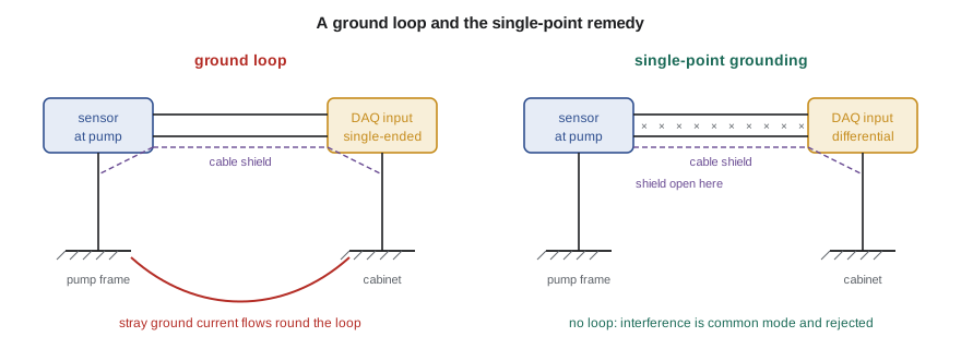
The remedies are to break the loop or to make the measurement immune to it. A differential input measures between the signal's two wires rather than between one wire and the local ground, so a voltage between grounds appears as common mode and is rejected. Shields are grounded at one end only, normally the instrument end, so no current flows in them; the exception is very high frequency interference, for which shields may need to be bonded at both ends through the connector shell, and drive manufacturers often require this for motor cables. Isolation amplifiers, which pass the signal through a transformer, optical or capacitive barrier, break the loop completely.
One rule overrides all the others. The protective, or safety, ground connections of equipment must never be removed to cure a noise problem. Those connections exist so that a fault cannot leave a metal frame live, and electrical codes require them, in the United States through the National Electrical Code and OSHA's electrical safety rules. Lifting a safety ground can turn a noise problem into a fatal shock hazard. Signal grounding is arranged within the instrumentation, using differential inputs, isolation and single-point signal commons, without touching the protective earthing.
Curing the TL-3 torque noise
Gilles and Owen find three faults. The torque transducer's signal cable runs for six meters in the same cable tray as the VFD's motor cable. Its shield is bonded both at the transducer and at the cabinet. And the transducer's conditioner is set for single-ended output into the data acquisition input. They move the signal cable to a separate tray, crossing the power cables at right angles where it must, ground its shield only at the cabinet, set the conditioner and input to differential, and set the input filter to 10 Hz for steady testing. The fuzzy band collapses to a scatter of ±0.03 N·m, and the torque's random contribution, which had threatened the budget of Lesson 3, becomes negligible.
Worked problem
Choosing an amplifier gain
A load cell rated at 2.0 mV/V full scale is excited at 10 V and feeds a data acquisition input of ±10 V range. The largest load expected is 70 percent of rated capacity, and Gilles wants 25 percent headroom above it. What gain should the instrumentation amplifier have?
Show solution
- Full-scale output: \(2.0 \times 10 = 20\) mV.
- Largest expected output: \(0.70 \times 20 = 14\) mV.
- With 25 percent headroom the largest output should be \(10/1.25 = 8\) V, so \(G = 8/0.014 = 571\).
Answer: A gain of about 570, or the nearest standard setting below it, uses most of the input range while leaving room for overloads and transients.
Common mistakes
MistakeUsing a single-ended input for a bridge or thermocouple signal in an industrial cell.
InsteadUse differential inputs so ground voltage differences are rejected.
MistakeGrounding a cable shield at both ends by default.
InsteadGround signal shields at one end unless high-frequency practice or the maker's instructions say otherwise.
MistakeRunning signal cables in the same tray as drive output cables.
InsteadSeparate them and cross at right angles.
MistakeDisconnecting a protective ground to stop hum.
InsteadNever; cure the noise with differential inputs, isolation or rewiring.
MistakeFiltering heavily without recording the filter setting.
InsteadRecord the filter type and cutoff with the data; it changes the dynamic response.
Summary and key terms
- Signal conditioning supplies excitation and converts, amplifies, filters, isolates and linearizes sensor signals.
- A Wheatstone bridge measures small resistance changes against zero; half and full bridges double and quadruple the output.
- Bridge sensitivities are quoted in mV/V; ratiometric measurement and sense leads remove excitation errors.
- Instrumentation amplifiers reject common-mode voltage; CMRR of 120 dB rejects a million to one.
- Interference couples capacitively, inductively and through shared grounds; separation, twisting, shielding and differential inputs cure it.
- Protective grounds are never removed to cure noise.
- Signal conditioning
- Circuits that convert a sensor's output into a clean signal suited to recording.
- Wheatstone bridge
- Four resistances in a diamond whose output measures small changes in one or more arms.
- Excitation
- The voltage or current supplied to a passive sensor so it can produce an output.
- Ratiometric measurement
- Dividing a bridge output by the excitation measured at the same time.
- Instrumentation amplifier
- A precision differential amplifier with high input impedance and high common-mode rejection.
- Common-mode rejection ratio
- The ratio of differential gain to common-mode gain of an amplifier.
- Thermal noise
- Random voltage generated in any resistance by the thermal motion of electrons.
- Ground loop
- A closed conducting path through two or more ground connections that lets stray currents add voltage to a signal.
- Shield
- A conducting layer around signal conductors that intercepts electric-field interference.
- Isolation amplifier
- An amplifier that passes a signal across an insulating barrier, breaking ground connections.
Practice problems
Work each problem on paper first, then reveal the answer to check.
A quarter-bridge strain gauge with GF 2.1 sees 800 microstrain with 5 V excitation. Find the output.
Show answer
x = 1.68e-3; Vo ≈ 5 × 1.68e-3/4 = 2.10 mV.
How much larger is the output of a full bridge than a quarter bridge for the same strain magnitude?
Show answer
Four times.
In the program, what would a second-order filter pass at 60 Hz with a 10 Hz cutoff?
Show answer
1/√(1 + 6⁴) = 0.028, or about −31 dB.
Why does narrowing the bandwidth from 10 kHz to 10 Hz reduce thermal noise?
Show answer
Thermal noise voltage is proportional to √B, so it falls by √1000 ≈ 32 times.
A signal cable picks up hum that disappears when the motor stops but not when the drive is bypassed. Which coupling path is most likely?
Show answer
Inductive coupling from the motor current, since the hum follows the current rather than the drive's switching.
Lesson quiz · 5 questions
Score 60% or more to complete this lesson.
Create a free account to save your progress, take quizzes and earn a certificate.