
MEC-395 · Lesson 12 of 12 · 22 min
Test planning and the pump performance test capstone
Everything in this course comes together on the morning of the witnessed test. The customer's inspector has traveled to Portland to watch the sixth TP-80 of the order, serial number 6, run on TL-3; Marco Rossi will sign the certificate; Lucie Arsenault is the test engineer of record and Owen Clarke runs the stand. A test of this kind is an experiment with a defined purpose, and like any experiment it succeeds or fails largely before it begins, in the planning. This lesson covers how tests and experiments are planned, how the TP-80 test is run and reduced, and how its result is judged against the guarantee.
Planning an experiment
Every test starts with a clear statement of its objective, because the objective decides what is measured, how well and at which conditions. The objective of the witnessed test is narrow: to show, with a stated uncertainty, whether the pump meets its guaranteed head and efficiency at 90 m³/h and 1,760 rpm, and to record its curve over the whole flow range. A development test would have a different objective, such as finding which of three impeller designs is most efficient, and would be planned differently.
From the objective follow the measurands, the instruments and the uncertainty each must achieve, which is where the budget of Lesson 3 is used in reverse: Owen starts from the uncertainty the result needs and works back to what each instrument must deliver. Then come the test conditions and their order, the number of readings at each, the criteria for steady conditions, the data reduction, the acceptance criteria and the report. Writing these down as a test procedure, agreed with the customer before the test, avoids arguments afterwards about what was meant.
Variables and the design of experiments
Experiments involve independent variables, which the experimenter sets, such as valve position or speed; dependent variables, which are measured, such as head and torque; and extraneous variables, which also affect the results but are not of interest, such as water temperature, ambient temperature, supply voltage and the operator. Good experimental design controls extraneous variables where it can, measures them where it cannot, and arranges the tests so that whatever is left over does not masquerade as an effect of the independent variables.
Three principles do most of the work. Replication, repeating runs, estimates the random scatter and reduces its effect on averages, as in Lesson 2. Randomization, running conditions in a random order, prevents slow drifts, such as the water warming or an instrument drifting, from lining up with the planned sequence of conditions. Blocking groups runs made under similar conditions, such as the same day or the same water fill, so that differences between groups can be separated from the effects under study. When several factors may matter, a factorial design varies them together rather than one at a time, so that their interactions can be seen.
Worked problem
A two-factor experiment on the test stand
Before the order's first test, Owen wants to know whether water temperature (15 or 35 °C) and suction pressure (1.05 or 1.30 bar absolute) affect the efficiency measured at the guarantee point. He runs all four combinations twice, in random order, and obtains these mean efficiencies: 15 °C and 1.05 bar, 75.81 percent; 35 °C and 1.05 bar, 75.93; 15 °C and 1.30 bar, 75.84; 35 °C and 1.30 bar, 75.95. The standard deviation of single runs is 0.06 points. What are the main effects and the interaction, and are any significant?
Show solution
- Temperature effect: average at 35 °C minus average at 15 °C, \((75.93 + 75.95)/2 - (75.81 + 75.84)/2 = 0.115\) points.
- Suction pressure effect: \((75.84 + 75.95)/2 - (75.81 + 75.93)/2 = 0.025\) points. Interaction: \(\big((75.95 - 75.84) - (75.93 - 75.81)\big)/2 = -0.005\) points.
- Each effect is a difference of two averages of four runs, so its standard deviation is \(0.06\sqrt{1/4 + 1/4} = 0.042\) points; about twice that, 0.085, is the threshold for significance at roughly 95 percent.
Answer: Only temperature has a significant effect, about 0.12 points over 20 °C, consistent with lower water viscosity reducing friction losses at higher temperature. Suction pressure, in this range, has none. The test procedure therefore specifies the water temperature band and reports the temperature with the results.
The test matrix and steady conditions
The pump test standards ask for a minimum number of points spread over the flow range, with points close to the guarantee point, so that the curve can be interpolated there. Owen's matrix has seven points: shut-off, 30, 55, 75, 90, 105 and 120 m³/h, about 0 to 133 percent of rated flow. The order is not simply ascending; he runs 90 m³/h first, then the others in a shuffled order, and 90 m³/h again at the end, so that any drift during the test shows up as a difference between the two guarantee-point readings. Shut-off is run briefly, because the water in the pump heats quickly with no flow through it.
At each point the stand must reach steady conditions before readings are taken. Owen's software applies the criterion in the procedure: after the valve and speed settle, the two-second averages of flow, pressures, torque and speed must stay within stated small bands for one minute, and the readings are then logged for one more minute, giving the thirty readings that Lesson 2 showed were needed. The software also checks every channel's calibration date and loop current, flags any reading that fails the outlier screen of Lesson 2 for the operator to explain, and records the water temperature and the barometer with every point.
Data reduction
Raw readings become results through the chain built over the course: the flowmeter factor of Lesson 10 corrects the flow; the head equation of Lesson 8 combines the pressures, barometer, heights and velocities; torque and speed give shaft power; and efficiency follows. Because the speed at each point differs slightly from rated speed, the results are corrected to 1,760 rpm by the affinity laws, with flow scaled by the speed ratio, head by its square and power by its cube, while efficiency is unchanged. The test standards permit such corrections only when the test speed is within a modest band of the rated speed, because the laws are exact only for geometrically and dynamically similar conditions.
# Capstone: reduce the witnessed test of TP-80 serial 6, correct to rated speed and judge the guarantee
import math
g, n0 = 9.807, 1760.0
rho = 998.2                                       # water at 20.0 C throughout (TT-102)
pb = 1.0130e5
Ds, Dd, dz = 0.125, 0.100, 0.200
# Test points: flow m3/h (FT-201 x meter factor), discharge bar g, suction bar abs, torque N m, speed rpm
raw = [(0.00, 4.0040, 1.1352, 19.50, 1758.6), (29.99, 3.9370, 1.1345, 34.30, 1759.2), (55.01, 3.7380, 1.1331, 45.20, 1760.4),
       (75.04, 3.4950, 1.1316, 51.80, 1761.0), (90.08, 3.2400, 1.1300, 56.80, 1760.0), (104.97, 2.9550, 1.1280, 60.70, 1759.5),
       (119.92, 2.6200, 1.1257, 64.00, 1758.8)]
# Relative standard uncertainties (from Lessons 3, 7, 8, 10, 11): flow, head, torque, speed
uQ, uH, uT, un = 0.00125, 0.00066, 0.00102, 0.00033
pts = []
print("   Q(test)  n(test)   Q(1760)  H(1760)  P(1760)   eta     U(eta), k = 2")
for Q, pd, ps, T, n in raw:
    q = Q/3600; v1 = q/(math.pi*Ds**2/4); v2 = q/(math.pi*Dd**2/4)
    H = ((pd*1e5 + pb) - ps*1e5)/(rho*g) + dz + (v2*v2 - v1*v1)/(2*g)
    P = 2*math.pi*n/60*T
    r = n0/n                                      # affinity-law correction to rated speed
    Qc, Hc, Pc = Q*r, H*r*r, P*r**3
    e = rho*g*q*H/P if Q > 0 else 0.0
    Ue = 2*e*math.sqrt(uQ**2 + uH**2 + uT**2 + un**2)
    pts.append((Qc, Hc, Pc, e))
    print(f"  {Q:7.2f}  {n:7.1f}   {Qc:7.2f}   {Hc:6.2f}   {Pc/1000:6.2f}   {100*e:5.2f}    +/-{100*Ue:.2f}")
# Interpolate the corrected curves at the guarantee flow of 90 m3/h (quadratic through the three nearest points)
def quad(xs, ys, x):
    return sum(ys[i]*math.prod((x - xs[j])/(xs[i] - xs[j]) for j in range(3) if j != i) for i in range(3))
near = pts[3:6]
Hg = quad([p[0] for p in near], [p[1] for p in near], 90.0)
eg = quad([p[0] for p in near], [p[3] for p in near], 90.0)
xs, ys = [p[0] for p in near], [p[1] for p in near]
slope = (quad(xs, ys, 90.5) - quad(xs, ys, 89.5))/1.0          # dH/dQ, m per m3/h
# head itself, the speed correction (H scales with n squared) and the flow uncertainty moving us along a sloping curve
UH = 2*math.sqrt((Hg*uH)**2 + (Hg*2*un)**2 + (slope*90.0*uQ)**2)
Ue = 2*eg*math.sqrt(uQ**2 + uH**2 + uT**2 + un**2)
print(f"\nSlope of the head curve at 90 m3/h: {slope:.3f} m per m3/h")
print(f"At the guarantee flow of 90.0 m3/h: H = {Hg:.2f} m +/- {UH:.2f} m, efficiency {100*eg:.2f} % +/- {100*Ue:.2f} points (k = 2)")
H_g, H_tol, e_g = 32.0, 0.03, 0.750                 # contract: 32.0 m with -0/+3 %, efficiency at least 75.0 %
print(f"Head band {H_g:.2f} to {H_g*(1 + H_tol):.2f} m:", "inside" if H_g <= Hg <= H_g*(1 + H_tol) else "outside",
      f"(margin to the nearer limit {min(Hg - H_g, H_g*(1 + H_tol) - Hg):.2f} m, against U = {UH:.2f} m)")
print(f"Efficiency {100*eg:.2f} % against {100*e_g:.1f} %: margin {100*(eg - e_g):.2f} points, {((eg - e_g)/Ue):.1f} times U")
best = max(pts, key=lambda p: p[3])
print(f"Best measured efficiency {100*best[3]:.2f} % near {best[0]:.0f} m3/h; shut-off head {pts[0][1]:.2f} m at 1,760 rpm") Q(test) n(test) Q(1760) H(1760) P(1760) eta U(eta), k = 2
0.00 1758.6 0.00 39.92 3.60 0.00 +/-0.00
29.99 1759.2 30.00 39.25 6.33 50.60 +/-0.18
55.01 1760.4 55.00 37.25 8.33 66.91 +/-0.24
75.04 1761.0 75.00 34.86 9.54 74.56 +/-0.26
90.08 1760.0 90.08 32.41 10.47 75.83 +/-0.27
104.97 1759.5 105.00 29.64 11.19 75.61 +/-0.27
119.92 1758.8 120.00 26.39 11.81 72.91 +/-0.26
Slope of the head curve at 90 m3/h: -0.174 m per m3/h
At the guarantee flow of 90.0 m3/h: H = 32.42 m +/- 0.07 m, efficiency 75.83 % +/- 0.27 points (k = 2)
Head band 32.00 to 32.96 m: inside (margin to the nearer limit 0.42 m, against U = 0.07 m)
Efficiency 75.83 % against 75.0 %: margin 0.83 points, 3.1 times U
Best measured efficiency 75.83 % near 90 m3/h; shut-off head 39.92 m at 1,760 rpmResults
The program reduces the seven points. At rated speed the pump develops 39.9 m at shut-off and 26.4 m at 120 m³/h, with its best efficiency, 75.8 percent, close to the guarantee flow. Interpolating the corrected curves at exactly 90.0 m³/h gives a head of 32.42 m and an efficiency of 75.83 percent. The final repeat of the guarantee point, not shown in the table, agreed with the first within 0.02 m and 0.04 points, so no drift occurred.
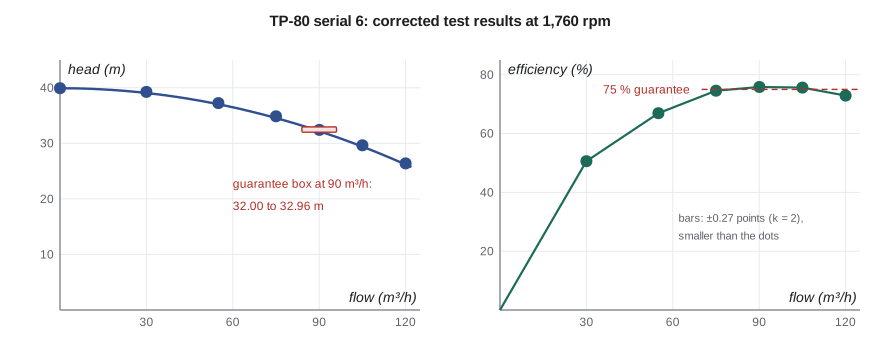
The uncertainty at the guarantee flow combines the contributions found in the earlier lessons. For efficiency it is ±0.27 points at k = 2, as in Lesson 3. For head it is ±0.07 m, which includes not only the pressure measurement but also the speed correction, since head scales with the square of speed, and the flow uncertainty, which matters because the head curve slopes: an error of 0.11 m³/h in flow places the reading at a slightly wrong point on a curve falling 0.17 m per m³/h. These are the numbers the test standards ask the laboratory to show are within their permissible limits; for the most demanding grade, those limits are tight, of the order of a percent or two on flow and efficiency, and TL-3's budget meets them with a clear margin.
Judging conformity
The purchase order applies an acceptance grade of the test standard, and for this order the agreed criteria are a head at the guarantee flow between 32.0 m and 3 percent above it, and an efficiency no lower than 75.0 percent. The measured head of 32.42 m lies 0.42 m inside the nearer limit, six times its expanded uncertainty. The efficiency of 75.83 percent exceeds its limit by 0.83 points, more than three times its expanded uncertainty. Both results conform clearly.
The decision would be harder if a result lay close to a limit. A decision rule, agreed in advance, says how the uncertainty is used. Under simple acceptance, a result inside the limit passes whatever its uncertainty; under guarded acceptance, the result must be inside the limit by at least a guard band, often the expanded uncertainty, so that the risk of wrongly passing a non-conforming pump is small. Guarded acceptance protects the buyer at the cost of rejecting some good pumps; simple acceptance shares the risk. International guidance for accredited laboratories asks that the decision rule be stated when a statement of conformity is given. For this order the purchase contract adopts the test standard's own approach, under which the tolerances already allow for measurement uncertainty, and the laboratory states its uncertainty alongside.
| Quantity at 90.0 m³/h | Measured | Expanded uncertainty (k = 2) | Acceptance limit | Margin | Result |
|---|---|---|---|---|---|
| Total head | 32.42 m | ±0.07 m | 32.00 to 32.96 m | 0.42 m | Conforms |
| Efficiency | 75.83 % | ±0.27 points | at least 75.0 % | 0.83 points | Conforms |
| Shaft power | 10.46 kW | ±0.02 kW | information only | not applicable | Reported |
The report and the certificate
The test report records everything needed to repeat and check the result: the pump's identity and configuration, the stand and its layout, every instrument with its calibration reference and due date, the test procedure and any deviations from it, the raw readings, the data reduction method, the corrected results, the uncertainty budget and the decision rule, and the signatures of those responsible. The certificate that goes to the customer summarizes the results and the conformity statement, refers to the report, and is signed by Marco. The customer's inspector signs the witness record. All six pumps of the order have now been tested, and all conform.
Owen reflects that the result itself, a curve and two ticks, is the smallest part of the work. The calibration of PT-210 with its zero trim, the outlier that turned out to be a moving valve, the torque noise cured by rerouting a cable, the vented impulse lines, the weigh-tank buoyancy correction and the period timing of speed each removed an error that could have spoiled the result without anyone noticing. Measurement is a chain, and its strength is that of its weakest link.
Common mistakes
MistakeRunning test points in ascending order only.
InsteadShuffle the order and repeat the guarantee point at the end to reveal drift.
MistakeTaking readings before the stand has settled.
InsteadApply a stated steady-state criterion before logging.
MistakeVarying one factor at a time when factors may interact.
InsteadUse a factorial design to see main effects and interactions.
MistakeApplying affinity-law corrections over a wide speed range.
InsteadKeep test speed within the band the standard allows.
MistakeStating conformity without a decision rule.
InsteadAgree in advance how uncertainty is used in the pass or fail decision.
Summary and key terms
- A test plan follows from its objective: measurands, instruments, uncertainty targets, matrix, steady-state criteria, reduction and acceptance.
- Replication, randomization and blocking control extraneous variables; factorial designs reveal interactions.
- Results are corrected to rated speed by the affinity laws: Q ∝ n, H ∝ n², P ∝ n³, efficiency unchanged.
- At 90.0 m³/h serial 6 gave H = 32.42 ± 0.07 m and η = 75.83 ± 0.27 percent (k = 2).
- Both results conform with margins several times their uncertainties.
- A decision rule, simple or guarded, states how uncertainty enters a conformity decision.
- Test objective
- The question a test is designed to answer, which determines what and how well to measure.
- Independent variable
- A variable set by the experimenter.
- Extraneous variable
- A variable that affects the results but is not under study.
- Replication
- Repeating runs to estimate and reduce random scatter.
- Randomization
- Running conditions in random order so drifts do not mimic effects.
- Blocking
- Grouping runs made under similar conditions to separate group differences from effects.
- Factorial design
- An experiment in which factors are varied together in all combinations.
- Affinity laws
- Scaling relations giving flow, head and power of a pump at a different speed.
- Decision rule
- The rule stating how measurement uncertainty is accounted for in a statement of conformity.
- Guard band
- A margin inside a tolerance limit required for acceptance to reduce the risk of a wrong pass.
Practice problems
Work each problem on paper first, then reveal the answer to check.
A point measured at 1,752 rpm gives 88.0 m³/h and 32.1 m. Correct it to 1,760 rpm.
Show answer
Q = 88.0 × 1.00457 = 88.40 m³/h; H = 32.1 × 1.00916 = 32.39 m.
Shaft power at 1,752 rpm is 10.30 kW. What is it at 1,760 rpm?
Show answer
10.30 × 1.00457³ = 10.44 kW.
In the program, what would the head margin be if the guarantee were 32.3 m?
Show answer
0.12 m, still above the expanded uncertainty of 0.07 m.
Under guarded acceptance with a guard band equal to U, would an efficiency of 75.20 ± 0.27 percent pass a 75.0 percent limit?
Show answer
No; it must be at least 75.27 percent.
Why is the guarantee point repeated at the end of the test?
Show answer
A change between the two readings reveals drift in the stand or the pump during the test.
Lesson quiz · 5 questions
Score 60% or more to complete this lesson.
Create a free account to save your progress, take quizzes and earn a certificate.