
MEC-395 · Lesson 10 of 12 · 22 min
Flow measurement
Flow rate contributed half the variance in Lesson 3's efficiency budget, so it deserves the most attention of any measurement on TL-3. The stand measures flow with FT-201, an electromagnetic flowmeter, and calibrates that meter in place against WT-1, the weigh tank, by collecting water for a timed interval. This lesson surveys the main kinds of flowmeter, explains how each works and where it fails, and then follows Owen and Gilles through the weigh-tank calibration that gives FT-201 its traceability.
Volume flow, mass flow and the velocity profile
Volume flow rate Q is the volume passing a section per unit time; mass flow rate is \(\dot{m} = \rho Q\). Pump performance is stated in volume flow, but the most accurate primary method, weighing, measures mass, so density must be known to convert. Most flowmeters do not measure flow directly at all. They measure a velocity, a velocity-dependent pressure or a velocity-dependent signal at some part of the pipe section, and rely on the velocity profile across the pipe to be the one assumed in their calibration. A fully developed turbulent profile in a long straight pipe is fairly flat; downstream of an elbow, a valve or a pump it is skewed and swirling, and most meters then read wrongly. Every flowmeter specification therefore comes with straight-length requirements, a number of pipe diameters of straight pipe needed upstream and downstream, and meeting them is as important as choosing the meter.
Differential-pressure meters
The oldest industrial flowmeters place a restriction in the pipe and measure the pressure drop it causes. By Bernoulli's equation, accelerating the flow through a smaller area lowers its pressure in proportion to the square of the velocity, so for an orifice plate of bore d in a pipe of diameter D, with diameter ratio \(\beta = d/D\),
where C is the discharge coefficient, which accounts for the contraction of the jet and friction, and ε is the expansibility factor, equal to one for liquids. The international standard ISO 5167 specifies the geometry of orifice plates, nozzles and Venturi tubes, the positions of their pressure tappings and the required straight lengths, and gives empirical equations for C. A meter built and installed to the standard can be used without flow calibration with an uncertainty of the order of half a percent to one percent, which is its great attraction.
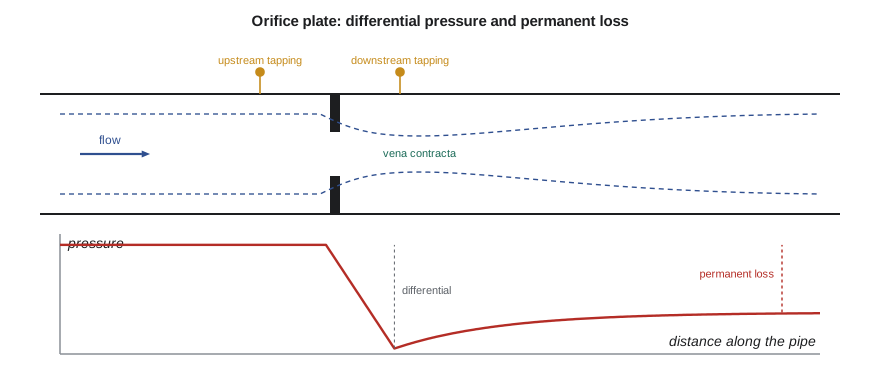
Differential-pressure meters have two weaknesses. The first is their square-root law: at half the flow the differential is a quarter of full scale, and at 30 percent it is under a tenth, so the uncertainty grows rapidly at low flow and the usable range, or turndown, is limited to perhaps four or five to one with a single transmitter. The second is permanent pressure loss. An orifice plate wastes a large part of its differential as turbulence downstream; the program shows that an orifice sized for TL-3's 90 m³/h would cost nearly 6 m of head, a fifth of the pump's output. Venturi tubes, with their gradual contraction and long diffusing cone, recover most of the pressure but are long and expensive.
Velocity and volumetric meters
Electromagnetic flowmeters, or magmeters, apply Faraday's law of induction. Coils around a lined section of pipe create a magnetic field across the flow, and a conducting liquid moving through the field generates a voltage, proportional to its mean velocity, between two electrodes in the pipe wall. Magmeters have no moving parts and no obstruction, so they cause no pressure loss, they are insensitive to density and viscosity, and they are linear over a wide range. They need a liquid with some minimum electrical conductivity, which ordinary water easily has but hydrocarbons do not, and they are affected by severely distorted profiles, though less than many meters. A good magmeter, calibrated in a flow laboratory, is typically specified to about ±0.2 to 0.5 percent of reading over its upper range, which is why FT-201 was chosen.
Ultrasonic transit-time meters send pulses of sound diagonally across the pipe, alternately with and against the flow. The pulse traveling with the flow arrives slightly sooner, and the time difference is proportional to the velocity along the path. The program shows how small the effect is: across TL-3's 100 mm pipe at 3.2 m/s the difference is about 290 nanoseconds, and half a percent of flow is under 1.5 nanoseconds, so the electronics must time to picoseconds. Clamp-on ultrasonic meters, strapped to the outside of a pipe, are invaluable for checking flows in existing systems without cutting pipes, but their accuracy depends on knowing the pipe's wall thickness and inside diameter and on a good profile; a few percent is more likely than a few tenths. Multipath in-line ultrasonic meters, with several chordal paths, approach the accuracy of magmeters and are used for custody transfer of oil and gas.
Turbine meters use a free rotor whose speed is proportional to velocity, counted by a pickup; they are accurate and repeatable in clean liquids but have bearings that wear, and they are sensitive to viscosity and swirl. Vortex meters detect the vortices shed alternately from a bluff body in the flow, whose frequency is proportional to velocity. Positive-displacement meters trap and count discrete volumes of liquid and are the most accurate meters for viscous liquids such as oils.
Coriolis mass flowmeters
A Coriolis meter passes the flow through one or two tubes that are vibrated at their natural frequency. Fluid moving through a vibrating tube experiences Coriolis forces that twist the tube slightly, and the phase difference between the motion of its inlet and outlet ends is proportional to mass flow rate. The tube's natural frequency also gives the fluid's density. Coriolis meters measure mass directly, independent of the velocity profile, and they are among the most accurate flowmeters available, often ±0.1 percent of reading for liquids. Their limits are size, cost and pressure drop in large lines; for TL-3's 100 mm line a Coriolis meter would be large and expensive, but for the small-pump stand next door it is the meter of choice.
| Meter type | Principle | Typical uncertainty | Pressure loss | Main limitations |
|---|---|---|---|---|
| Orifice plate | Differential pressure | About 0.5 to 1 % to ISO 5167 | High | Square-root turndown; long straight runs |
| Venturi tube | Differential pressure | About 0.5 to 1 % | Low | Size and cost |
| Electromagnetic | Faraday induction | About 0.2 to 0.5 % of reading | None | Conducting liquids only |
| Ultrasonic transit time | Sound transit time | 0.5 % (multipath) to a few % (clamp-on) | None | Profile, pipe dimensions |
| Turbine | Rotor speed | About 0.25 to 0.5 % | Moderate | Wear, viscosity, swirl |
| Coriolis | Tube twist from Coriolis force | About 0.1 % of reading | Moderate to high | Size and cost in large lines |
Primary calibration: the weigh tank
A flowmeter's calibration must ultimately trace to the base units of mass or length and time. The most accurate method for liquids is gravimetric: the flow is collected in a tank on a weighing system for a measured time. On TL-3 a diverter, a swinging nozzle at the end of the return line, switches the flow between the return to the suction tank and the weigh tank. The time of collection is measured by a timer triggered by the diverter's motion, so that it starts and stops at the moment the stream crosses the dividing edge. Errors in diverter timing are the classic weakness of the method, because the stream takes a finite time to cross; a well-designed diverter crosses quickly and symmetrically, and its timing error is checked by varying the collection time.
The weighed mass needs two corrections. The span factor from the test-weight check of Lesson 7 corrects the weighing system. Buoyancy must also be considered: the water in the tank displaces air, and so do the steel test weights that calibrated the tank, but water displaces much more air per kilogram than steel does. The true mass of water is therefore slightly greater, by about 0.1 percent, than the reading of a scale calibrated with steel weights. Volume then follows from mass and the density of water at the measured temperature.
# Flow measurement: weigh-tank calibration of FT-201, an orifice-plate comparison and a transit-time ultrasonic meter
import math
# 1. Static gravimetric calibration: flow diverted into WT-1 for a timed collection
rho_w, rho_air, rho_ref = 998.2, 1.2, 8000.0     # water at 20 C, air, reference density of the test weights
span = 1.00070                                   # span factor from the test-weight check (Lesson 7)
runs = [  # (indicated mass change kg, diverter time s, FT-201 totalized volume m3)
    (3005.6, 120.02, 3.0172), (3008.9, 120.15, 3.0204), (3003.1, 119.95, 3.0151)]
factors = []
print(" run   mass (kg)  time (s)  volume ref (m3)  meter (m3)   ref flow (m3/h)  meter error")
for k, (mi, t, vm) in enumerate(runs, 1):
    m = mi*span*(1 - rho_air/rho_ref)/(1 - rho_air/rho_w)   # buoyancy: weighed in air against steel-density weights
    V = m/rho_w; qref = V/t*3600; err = 100*(vm - V)/V; factors.append(V/vm)
    print(f"  {k}    {mi:8.1f}   {t:7.2f}      {V:8.4f}       {vm:7.4f}       {qref:7.2f}        {err:+.3f} %")
mf = sum(factors)/len(factors)
s = math.sqrt(sum((f - mf)**2 for f in factors)/(len(factors) - 1))
print(f"Meter factor {mf:.5f} (repeatability s = {100*s:.3f} %, standard error {100*s/math.sqrt(len(factors)):.3f} %)")
# 2. Orifice plate in the 100 mm line, beta 0.60, discharge coefficient about 0.605 (ISO 5167 gives it precisely)
D, beta, Cd = 0.100, 0.60, 0.605
d = beta*D; Ao = math.pi*d*d/4
q = 90.08/3600
dp = rho_w/2*(q*math.sqrt(1 - beta**4)/(Cd*Ao))**2
loss = (1 - beta**1.9)*dp
print(f"\nOrifice, d = {d*1000:.1f} mm: differential {dp/1000:.1f} kPa at 90 m3/h; permanent loss about {loss/1000:.1f} kPa ({loss/(rho_w*9.807):.2f} m of head)")
for frac in (1.0, 0.5, 0.3):
    print(f"  at {100*frac:3.0f} % of the flow the differential is {100*frac**2:5.1f} % of full")
# 3. Transit-time ultrasonic meter, clamped on at 45 degrees across the same pipe
c, theta = 1482.0, math.radians(45)
v = q/(math.pi*D*D/4); Lp = D/math.sin(theta)
dt = 2*Lp*v*math.cos(theta)/c**2
print(f"\nUltrasonic: mean velocity {v:.3f} m/s, path {Lp*1000:.0f} mm, upstream-downstream time difference {dt*1e9:.1f} ns")
print(f" 0.5 % of flow corresponds to {0.005*dt*1e12:.0f} ps")run mass (kg) time (s) volume ref (m3) meter (m3) ref flow (m3/h) meter error 1 3005.6 120.02 3.0163 3.0172 90.47 +0.030 % 2 3008.9 120.15 3.0196 3.0204 90.48 +0.026 % 3 3003.1 119.95 3.0138 3.0151 90.45 +0.043 % Meter factor 0.99967 (repeatability s = 0.009 %, standard error 0.005 %) Orifice, d = 60.0 mm: differential 93.0 kPa at 90 m3/h; permanent loss about 57.7 kPa (5.90 m of head) at 100 % of the flow the differential is 100.0 % of full at 50 % of the flow the differential is 25.0 % of full at 30 % of the flow the differential is 9.0 % of full Ultrasonic: mean velocity 3.186 m/s, path 141 mm, upstream-downstream time difference 290.1 ns 0.5 % of flow corresponds to 1451 ps
Three collections of about two minutes and three metric tons each give reference flows near 90.5 m³/h and show FT-201 reading 0.03 to 0.04 percent high. The meter factor is 0.99967, with a repeatability of 0.009 percent, so the three runs agree very closely. Gilles enters the factor into the data acquisition software rather than adjusting the meter, so that the meter's own setting and the correction are both visible. Owen's uncertainty budget for the calibration includes the weighing system and test weights, the buoyancy correction, the density of water from TT-102, diverter timing and repeatability; it comes to about 0.12 percent at k = 2, and with the flowmeter's own behavior between calibrations, the 0.25 percent used in Lesson 3 is a comfortably supported figure.
Calibration in place has an important advantage over sending the meter to a flow laboratory: it includes the actual installation, with its upstream bends and valves, so profile effects are part of the calibrated result. Its disadvantage is that the installation must not change afterwards. Gilles marks every flange in the measuring section, and any work on the upstream pipework triggers a recalibration.
Worked problem
Choosing a meter for a field check
A customer reports that a TP-80 in service delivers only about 75 m³/h. The pump discharges into a 100 mm steel line with an elbow 1.5 m upstream of the only accessible straight section. Owen has a clamp-on ultrasonic meter specified to ±1 percent of reading under ideal conditions. How confident can he be in a reading?
Show solution
- The straight section starts only 15 diameters downstream of an elbow; clamp-on meters typically ask for 10 to 20 diameters upstream, so the profile may still be distorted.
- The steel pipe's inside diameter and wall thickness must be measured; a 1 mm error in a 100 mm diameter is a 2 percent error in area.
- Installing the transducers in two orientations, 90° apart, and comparing readings shows whether the profile is skewed.
Answer: A sensible estimate of uncertainty is a few percent, not one percent. That is enough to confirm a shortfall from 90 to 75 m³/h, which is 17 percent, but not enough to say whether the pump has lost two or three percent of its performance.
Common mistakes
MistakeInstalling a flowmeter immediately downstream of a bend or valve.
InsteadRespect the straight-length requirements or calibrate in place.
MistakeUsing a differential-pressure meter far below its design flow.
InsteadIts differential falls with the square of flow; plan the turndown or use two transmitters.
MistakeConverting weighed mass to volume without buoyancy correction.
InsteadWater displaces more air than steel weights; the correction is about 0.1 percent.
MistakeTrusting a clamp-on reading to its datasheet accuracy.
InsteadPipe dimensions and profile usually dominate; estimate the uncertainty honestly.
MistakeChanging pipework near a calibrated meter without recalibrating.
InsteadIn-place calibration includes the installation, which must not change.
Summary and key terms
- Most meters infer flow from velocity and rely on the velocity profile; straight-length requirements protect it.
- Differential-pressure meters follow a square-root law, have limited turndown and, for orifices, large permanent loss.
- Magmeters are obstruction-free and accurate for conducting liquids; ultrasonic meters time differences of nanoseconds.
- Coriolis meters measure mass flow and density directly and are among the most accurate.
- Gravimetric calibration with a diverter and weigh tank is the primary method for liquids; span and buoyancy corrections apply.
- FT-201's meter factor is 0.99967, determined in place with a repeatability of 0.009 percent.
- Volume flow rate
- The volume of fluid passing a section per unit time.
- Velocity profile
- The distribution of velocity across a pipe section.
- Straight length
- The run of straight pipe required upstream and downstream of a meter.
- Discharge coefficient
- The ratio of actual to ideal flow through a differential-pressure device.
- Turndown
- The ratio of maximum to minimum flow over which a meter meets its accuracy.
- Electromagnetic flowmeter
- A meter that measures the voltage induced in a conducting liquid moving through a magnetic field.
- Transit-time ultrasonic meter
- A meter that measures the difference in sound travel time with and against the flow.
- Coriolis meter
- A meter that measures mass flow from the twist of a vibrating tube.
- Gravimetric calibration
- Calibration by weighing the fluid collected over a measured time.
- Diverter
- A device that switches flow quickly between a return path and a collection tank.
Practice problems
Work each problem on paper first, then reveal the answer to check.
An orifice meter reads 40 kPa at 60 m³/h. What differential corresponds to 30 m³/h?
Show answer
10 kPa, a quarter.
Water collected in a weigh tank reads 2,500.0 kg in 100.00 s. Ignoring buoyancy, what is the flow at 998.2 kg/m³?
Show answer
2.5045 m³ in 100 s, or 90.16 m³/h.
In the program, what meter error would run 2 show without the buoyancy correction?
Show answer
About +0.13 percent, since buoyancy raises the reference volume by about 0.1 percent.
Why is a magmeter unsuitable for measuring the flow of lubricating oil?
Show answer
Oil is not electrically conducting, so no voltage is induced.
A clamp-on meter assumes a 102.3 mm bore, but the true bore is 100.0 mm. Roughly what error results?
Show answer
Area ratio 1.047; the reading would be about 4.7 percent high, before profile effects.
Lesson quiz · 5 questions
Score 60% or more to complete this lesson.
Create a free account to save your progress, take quizzes and earn a certificate.