
MEC-395 · Lesson 1 of 12 · 26 min
Measurement systems, calibration and traceability
Owen Clarke spent his last work term at Tidewater Pump Works in Portland automating TL-3, the company's new closed-loop pump test stand. He has now come back as a junior engineer in the test and reliability group, and his first assignment is the other half of the same job. TL-3 can now hold a pump at any flow and pressure, but a test stand exists to produce numbers that a customer will pay for and a certificate will vouch for. Marco Rossi, who signs Tidewater's test certificates, puts it simply: a pump that is guaranteed to deliver 90 m³/h at 32 m of head with 75 percent efficiency has to be shown to do so, by measurements whose quality can be stated and defended.
Lucie Arsenault, who leads the group, hands Owen the instrument list for the stand and the customer's purchase order for six TP-80 pumps. The order calls for a witnessed performance test to the Hydraulic Institute's test standard, ANSI/HI 14.6, which is closely aligned with the international pump test standard ISO 9906. Both standards say how pump performance is to be measured and how much measurement uncertainty is allowed. Over the twelve lessons of this course Owen will work through every link in that chain: what the instruments do, how good they are, how their signals are conditioned and recorded, and how the final efficiency figure and its uncertainty are worked out. This lesson sets out the vocabulary and the foundations: what a measurement system is, how it is calibrated, and why every reading must trace back to a national standard.
The generalized measurement system
Every measurement, from a tire gauge to a laboratory interferometer, can be described by the same chain of functional stages. A sensing element, or primary sensor, responds to the quantity being measured, called the measurand. A strain gauge changes resistance when stretched; a thermocouple produces a voltage that depends on temperature; a diaphragm deflects under pressure. The sensor's output is rarely in a convenient form, so a signal-conditioning stage converts and amplifies it: a bridge circuit turns resistance change into voltage, an amplifier raises millivolts to volts, a filter removes noise. An output stage then indicates, records or transmits the result, whether that is a pointer on a dial, a number on a screen, a 4 to 20 mA current sent to a controller or a sample stored by a data acquisition system.
Thinking in stages matters because each stage contributes its own errors, and because each can be calibrated, replaced or improved separately. When a reading looks wrong, the experienced technician works along the chain: is the sensor seeing the measurand it is supposed to see, is the conditioning circuit working, is the recording correct? Gilles Thériault, the instrumentation technologist who wired TL-3, keeps a loop sheet for every channel, showing each stage from sensor to stored value with its range, scaling and calibration date.
The instruments on TL-3
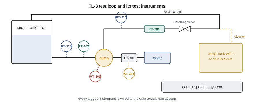
A pump performance test needs only a handful of quantities, but each must be measured well. Flow rate comes from a magnetic flowmeter in the discharge line, which is itself calibrated against a weigh tank that collects water for a timed interval. Pump head is calculated from pressures measured at the suction and discharge flanges, corrected for the heights of the gauges and for the velocity of the water. Power input to the pump is torque multiplied by rotational speed, measured by an in-line torque transducer between motor and pump. Water temperature sets the density and vapor pressure used in the calculations. Bearing-housing vibration and bearing temperature are recorded for the mechanical run test that many customers ask for alongside the performance test.
| Tag | Quantity | Instrument | Range | Stated accuracy |
|---|---|---|---|---|
| FT-201 | Flow rate | Magnetic flowmeter, DN 100 | 0 to 150 m³/h | ±0.3 % of reading above 1 m/s |
| PT-110 | Suction pressure | Piezoresistive transducer | 0 to 4 bar absolute | ±0.05 % of span |
| PT-210 | Discharge pressure | Piezoresistive transducer | 0 to 6 bar gauge | ±0.05 % of span |
| TQ-301 | Shaft torque | Strain-gauge torque transducer | 0 to 100 N·m | ±0.1 % of full scale |
| ST-301 | Shaft speed | 60-tooth wheel and magnetic pickup | 0 to 4,000 rpm | ±1 rpm |
| TT-102 | Water temperature | Pt100 RTD in thermowell | 0 to 60 °C | ±0.15 °C (class A at 0 °C) |
| WT-1 | Collected mass | Weigh tank on four load cells | 0 to 8,000 kg | ±0.05 % of load |
| VT-401/402 | Vibration | Piezoelectric accelerometers | ±50 g | ±5 % sensitivity |
Words that mean something precise
Measurement has its own vocabulary, defined internationally in the International Vocabulary of Metrology (the VIM), and using it carefully avoids a great deal of confusion. The measurand is the quantity intended to be measured, and defining it carefully is the first step of any test: \"the pump's total head\" is not the same measurand as \"the pressure rise across the pump\", because head includes elevation and velocity terms. The error of a measurement is the difference between the measured value and the true value of the measurand. Since the true value can never be known exactly, the error can never be known exactly either; what can be stated is the uncertainty, a parameter that characterizes the dispersion of values that could reasonably be attributed to the measurand.
Accuracy describes how close a measurement is to the true value. It is a qualitative idea in the VIM, although manufacturers routinely quote \"accuracy\" figures that are really limits of error. Precision describes how closely repeated measurements agree with one another, regardless of whether they agree with the truth. A gauge that consistently reads 0.2 bar high is precise but not accurate; one whose readings scatter widely around the right value is accurate on average but not precise. Repeatability is the precision obtained when the same operator measures the same thing with the same instrument under the same conditions over a short time; reproducibility is the precision across different operators, instruments, laboratories or times.
Several terms describe an instrument's scale. The range is the set of values it is designed to measure, such as 0 to 6 bar; the span is the difference between the upper and lower limits, here 6 bar. Resolution is the smallest change in the measurand that produces a perceptible change in the indication: a display showing three decimal places of bar has a resolution of 1 mbar, even if its accuracy is far coarser. Sensitivity is the change in output per unit change in input, such as 2.667 mA per bar for a 0 to 6 bar, 4 to 20 mA transmitter. Threshold or dead band is the smallest input change that the instrument responds to at all.
| Term | Meaning | TL-3 example |
|---|---|---|
| Measurand | Quantity intended to be measured | Pump total head at the guarantee flow |
| Error | Measured value minus true value | PT-210 reading 3.006 bar when the tester applies 3.000 bar |
| Uncertainty | Dispersion of values reasonably attributed to the measurand | Head known within ±0.12 m at 95 % confidence |
| Systematic error | Component of error that stays constant or varies predictably | A zero offset of +3.8 mbar |
| Random error | Component that varies unpredictably between repeated readings | Flowmeter scatter of ±0.2 m³/h |
| Resolution | Smallest perceptible change in indication | 0.1 rpm on the speed display |
| Sensitivity | Output change per unit input | 2.667 mA per bar for PT-210 |
| Span | Upper minus lower range limit | 6 bar for PT-210 |
Systematic and random error
Errors are usually divided into two kinds. A systematic error stays the same, or changes in a predictable way, when a measurement is repeated: a zero offset, a span that is 0.2 percent high, a temperature sensor that reads low because heat leaks along its sheath. Repeating the measurement does not reveal a systematic error, because every repetition is wrong by the same amount. It can only be found by comparison with something better, which is what calibration does. A random error varies unpredictably from one reading to the next, from electrical noise, turbulence in the flow, small changes in the operator's reading of a scale, and countless other causes. Random errors reveal themselves through scatter, and their effect on an average shrinks as the number of readings grows, as Lesson 2 shows.
There is a third kind that is better called a mistake: a reading written down wrongly, a transducer connected to the wrong channel, a unit confused. Mistakes are not part of any uncertainty analysis; they are prevented by procedure, checked for by sanity tests and removed when found. A good test engineer builds in redundancy so that mistakes show up. On TL-3, Owen arranges for the discharge pressure to be read both by PT-210 and by a calibrated digital test gauge at the start of each test, and for the flowmeter reading to be compared with the stand's control flowmeter, so that a gross disagreement stops the test before a day is wasted.
Calibration
Calibration is the operation that, under specified conditions, establishes the relation between the values indicated by an instrument and the corresponding values provided by measurement standards, together with their uncertainties. In practice, a calibration applies known inputs to an instrument, records its outputs, and either reports the errors found or uses them to adjust the instrument. The known inputs come from a reference standard whose own uncertainty is much smaller than that of the instrument under test; a ratio of four or more between the two is a common rule of thumb, sometimes called the test uncertainty ratio.
A good calibration covers the whole range in which the instrument will be used, at several points, approached from both directions. Applying pressures going up and then coming down reveals hysteresis, the difference between readings at the same input approached from below and from above. Fitting a straight line through the results separates the overall offset and span error from the scatter about the line, which is the nonlinearity. Calibration records report the instrument's condition as found, before any adjustment, and as left, after it. The as-found results matter more than they might seem: if an instrument is found out of tolerance, every measurement made with it since its last calibration is in question, and a test laboratory must review those results.
# Calibration of the TL-3 discharge pressure transducer PT-210 (0 to 6 bar gauge, 4 to 20 mA)
# against a deadweight tester: five points up, five points down
applied = [0.0, 1.5, 3.0, 4.5, 6.0, 6.0, 4.5, 3.0, 1.5, 0.0]           # bar, from the tester
mA      = [4.006, 8.008, 12.011, 16.009, 20.004, 20.004, 16.013, 12.017, 8.012, 4.008]
span_p, span_I = 6.0, 16.0
# Ideal (nominal) line: I = 4 + 16 p / 6.  Error of each reading, in bar and in percent of span
print(" applied  reading  indicated   error     error")
print("  (bar)    (mA)     (bar)      (bar)   (% span)")
ind = []
for p, i in zip(applied, mA):
    pi = (i - 4.0) * span_p / span_I; ind.append(pi)
    print(f"  {p:5.2f}   {i:6.3f}   {pi:7.4f}   {pi - p:+7.4f}   {100*(pi - p)/span_p:+6.3f}")
# Least-squares straight line through all ten points: indicated = a + b * applied
n = len(applied); mx = sum(applied)/n; my = sum(ind)/n
b = sum((x - mx)*(y - my) for x, y in zip(applied, ind)) / sum((x - mx)**2 for x in applied)
a = my - b*mx
res = [y - (a + b*x) for x, y in zip(applied, ind)]
print(f"\nBest-fit line: indicated = {a:+.4f} + {b:.5f} x applied  (zero offset {a*1000:+.1f} mbar, span factor {b:.5f})")
print(f"Largest deviation from the best-fit line (nonlinearity): {100*max(abs(r) for r in res)/span_p:.3f} % of span")
hyst = max(abs(ind[k] - ind[n - 1 - k]) for k in range(n // 2))
print(f"Largest up-down difference (hysteresis): {hyst*1000:.1f} mbar = {100*hyst/span_p:.3f} % of span")
worst = max(abs(pi - p) for p, pi in zip(applied, ind))
spec = 0.05
print(f"Largest error against the nominal line: {100*worst/span_p:.3f} % of span; specification +/-{spec} % of span:",
      "PASS" if 100*worst/span_p <= spec else "ADJUST")
# As left: the technician trims the zero by the best-fit offset and re-checks
left = max(abs(pi - a - p) for p, pi in zip(applied, ind))
print(f"After a zero trim of {a*1000:.1f} mbar, largest error {100*left/span_p:.3f} % of span:",
"PASS" if 100*left/span_p <= spec else "ADJUST")applied reading indicated error error (bar) (mA) (bar) (bar) (% span) 0.00 4.006 0.0023 +0.0023 +0.038 1.50 8.008 1.5030 +0.0030 +0.050 3.00 12.011 3.0041 +0.0041 +0.069 4.50 16.009 4.5034 +0.0034 +0.056 6.00 20.004 6.0015 +0.0015 +0.025 6.00 20.004 6.0015 +0.0015 +0.025 4.50 16.013 4.5049 +0.0049 +0.081 3.00 12.017 3.0064 +0.0064 +0.106 1.50 8.012 1.5045 +0.0045 +0.075 0.00 4.008 0.0030 +0.0030 +0.050 Best-fit line: indicated = +0.0038 + 0.99987 x applied (zero offset +3.8 mbar, span factor 0.99987) Largest deviation from the best-fit line (nonlinearity): 0.049 % of span Largest up-down difference (hysteresis): 2.3 mbar = 0.038 % of span Largest error against the nominal line: 0.106 % of span; specification +/-0.05 % of span: ADJUST After a zero trim of 3.8 mbar, largest error 0.042 % of span: PASS
Gilles calibrates PT-210 against the group's deadweight tester, an instrument that generates a known pressure by loading calibrated masses onto a piston of known area. The program shows the results. As found, the transducer reads up to 0.106 percent of span high, outside its specification of ±0.05 percent. Most of that is a zero offset of +3.8 mbar; the line through the points has a slope of 0.99987, almost exactly the nominal value, and the scatter about the line, the nonlinearity, is only 0.049 percent of span. Hysteresis is 2.3 mbar. Gilles trims the zero, rechecks, and the largest error falls to 0.042 percent of span, within specification. The as-found result is recorded, and because the offset is small compared with the head measurement's overall uncertainty, Lucie decides no earlier tests need to be reviewed. Lesson 8 returns to the deadweight tester and shows that even it needs a correction for local gravity.
Worked problem
Choosing a calibration standard
PT-210 must be verified to ±0.05 percent of its 6 bar span. The group has a digital test gauge with a stated uncertainty of ±0.02 percent of its 10 bar span, and a deadweight tester with a stated uncertainty of ±0.008 percent of reading. Which is suitable as the reference?
Show solution
- The tolerance to be verified is \(0.0005 \times 6 = 3.0\) mbar.
- The test gauge's uncertainty is \(0.0002 \times 10 = 2.0\) mbar, giving a ratio of \(3.0/2.0 = 1.5\).
- The deadweight tester's uncertainty is \(0.00008 \times 6 = 0.48\) mbar at full scale, giving a ratio above 6, and better still at lower pressures as a fraction of span.
Answer: Only the deadweight tester gives a ratio comfortably above four. The test gauge is fine for the daily cross-check against gross mistakes but not for calibration of PT-210.
Traceability
A calibration is only as good as the standard used for it, and that standard must itself have been calibrated against something better. Metrological traceability is the property of a measurement result whereby it can be related to a reference, usually the realization of an SI unit, through a documented, unbroken chain of calibrations, each contributing to the stated uncertainty. The masses of Tidewater's deadweight tester were calibrated by an accredited laboratory against its reference masses; those were calibrated against a national standard; and the national standard is tied to the definition of the kilogram, which since 2019 has been fixed through the Planck constant rather than a physical artifact. At each step the uncertainty grows a little, and the chain is only unbroken if every step is documented.
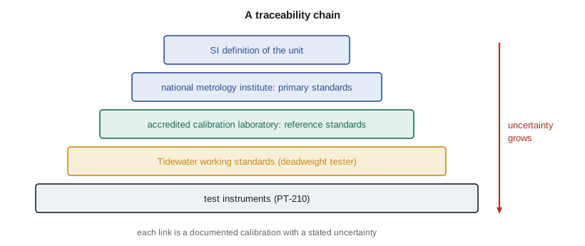
In the United States the top of the chain is the National Institute of Standards and Technology (NIST), the national metrology institute, which maintains the country's primary measurement standards and takes part in international comparisons with other national institutes. Calibration laboratories show their competence by accreditation to ISO/IEC 17025, the international standard for testing and calibration laboratories; accreditation bodies include the American Association for Laboratory Accreditation (A2LA), the ANSI National Accreditation Board (ANAB) and NIST's own National Voluntary Laboratory Accreditation Program (NVLAP). Weights and measures officials in each state, guided by NIST handbooks, regulate instruments used in trade, such as gasoline pumps and grocery scales, which is a different purpose from the engineering measurements of a test laboratory.
Accreditation bodies in different countries recognize one another's accreditations through international arrangements, so a calibration certificate from an accredited laboratory in one country is generally accepted in another. For Tidewater this matters because its customers are on both sides of the border, and a test certificate whose instruments trace to an accredited laboratory will be accepted by either. A calibration certificate worth the name states the instrument's identity, the method, the results with their uncertainties, the environmental conditions, the reference standards used and their traceability, and the date. A certificate that gives results without uncertainties, or names no reference, does not establish traceability, however official it looks.
Calibration intervals and records
Instruments drift, so calibration is repeated at intervals. There is no universal right interval; it depends on how stable the instrument has proved to be, how hard it is used, how critical its readings are, and what the standard or customer requires. A sensible approach is to start with the manufacturer's recommendation or the laboratory's usual practice, often one year for test transducers, and adjust it from experience: an instrument whose as-found results are always well within tolerance can have its interval lengthened, and one found out of tolerance should be checked more often. Between calibrations, simple intermediate checks, such as comparing two pressure transducers at the same tapping or reading the flowmeter at zero flow, catch drift early.
Tidewater keeps a record for each instrument with its identity, location, calibration history, as-found and as-left results, the certificate references and the next due date. The data acquisition system will not accept a channel whose calibration has expired, a rule Gilles programd after an embarrassing day early in his career when a test was run with an out-of-date torque meter. Owen adds one more field to every record: the uncertainty contributed by the instrument at TL-3's typical operating point, which he will need in Lesson 3 and again in the capstone.
Common mistakes
MistakeQuoting the resolution of a digital display as its accuracy.
InsteadResolution is only the smallest change shown; accuracy must come from calibration.
MistakeAssuming that repeating a measurement many times removes all error.
InsteadAveraging reduces random error only; systematic error is found by calibration against a better standard.
MistakeCalibrating an instrument with a reference only slightly better than itself.
InsteadAim for a reference whose uncertainty is a quarter or less of the tolerance being verified.
MistakeRecording only the as-left results of a calibration.
InsteadThe as-found results show whether earlier measurements were valid.
MistakeTreating any certificate as proof of traceability.
InsteadTraceability needs results with uncertainties and an unbroken, documented chain to national standards.
Summary and key terms
- A measurement system has sensing, signal-conditioning and output stages, each with its own errors.
- Error is unknowable exactly; uncertainty states the dispersion of values reasonably attributed to the measurand.
- Systematic errors are revealed only by calibration; random errors show as scatter and shrink when averaged.
- Calibration applies known inputs from a better standard, up and down the range, and reports as-found and as-left results.
- PT-210 was found 0.106 percent of span high, mostly a 3.8 mbar zero offset, and passed after a zero trim.
- Traceability is an unbroken, documented chain of calibrations to a national metrology institute, NIST, with uncertainty stated at every step.
- Measurand
- The quantity intended to be measured.
- Uncertainty
- A parameter that characterizes the dispersion of values that could reasonably be attributed to the measurand.
- Accuracy
- Closeness of a measured value to the true value of the measurand.
- Precision
- Closeness of agreement between repeated measurements.
- Resolution
- The smallest change in the measurand that produces a perceptible change in the indication.
- Sensitivity
- The change in an instrument's output per unit change in its input.
- Hysteresis
- The difference between readings at the same input approached from below and from above.
- Calibration
- Establishing the relation between an instrument's indications and values provided by measurement standards.
- Traceability
- The property of a result that relates it to a reference through an unbroken, documented chain of calibrations.
- ISO/IEC 17025
- The international standard for the competence of testing and calibration laboratories.
Practice problems
Work each problem on paper first, then reveal the answer to check.
A 4 to 20 mA transmitter covers 0 to 4 bar. What is its sensitivity?
Show answer
16 mA / 4 bar = 4.0 mA per bar.
In the program, what would the as-found largest error be if the zero offset were 1.0 mbar instead of the readings shown?
Show answer
Removing about 2.8 mbar from each error leaves about 3.6 mbar, or 0.06 percent of span, still just outside tolerance.
A thermometer reads 0.4 °C high at every point from 0 to 50 °C. Is this error random or systematic, and how would you find it?
Show answer
Systematic; only a comparison with a better reference, a calibration, will reveal it.
Why does a calibration approach each point from both directions?
Show answer
To reveal hysteresis, which a one-way calibration would hide.
A torque meter must be verified to ±0.1 N·m. What is the largest acceptable reference uncertainty for a 4:1 ratio?
Show answer
0.025 N·m.
Lesson quiz · 5 questions
Score 60% or more to complete this lesson.
Create a free account to save your progress, take quizzes and earn a certificate.