Quality, metrology, cost and lean manufacturing

The KG-40 is ready for launch. The housing pattern is approved, the gear forgings have passed their first-article inspection, the shaft cell is running, the cradle robot is programmed and the breather mold has been sampled. What remains is to show that every process can make good parts consistently, at the planned rate and cost, and to set up the systems that will keep it that way. This final lesson covers measurement, statistical process control and process capability, cost estimating, and the lean methods that remove waste from a production system. It ends with the launch plan the team presents to Kestrel Drive Systems's management.

Metrology: measuring what was made

A dimension is only known as well as it is measured. Metrology, the science of measurement, starts with traceability: every gauge is calibrated against a standard that is itself calibrated against higher standards, back to the national measurement institutes and the definition of the meter. Hand tools such as vernier and digital calipers resolve about 0.01 mm and suit general dimensions. Micrometers resolve 0.001 mm and suit diameters and thicknesses. Dial and digital indicators measure runout and flatness. Fixed gauges, such as go/no-go plug gauges for holes and ring or snap gauges for shafts, check whether a feature is within limits quickly, without giving a number. Surface plates, height gauges and gauge blocks provide reference planes and lengths.

Coordinate measuring machines (CMMs) move a touch probe or a scanning sensor in three axes and record points on the part, from which software computes sizes, positions, form errors and geometric tolerances against the CAD model and the GD&T on the drawing. Optical comparators, vision systems, laser scanners and X-ray computed tomography add non-contact options; CT can measure internal features and find porosity in castings and printed parts. In-process gauging on CNC machines and air gauges at grinders measure parts as they are made and feed corrections back to the machine.

A measuring system has its own variation. The rule of ten says a gauge should resolve about one tenth of the tolerance it checks. Gauge repeatability and reproducibility studies, in which several operators measure the same parts several times, separate the variation due to the gauge (repeatability) from that due to operators (reproducibility). If the measurement system uses up more than about 30 percent of the tolerance, its readings cannot tell good parts from bad reliably. Temperature matters too: the standard reference temperature for dimensional measurement is 20 °C, and a 300 mm steel shaft grows about 3.5 µm per degree.

Variation and statistical process control

No process makes identical parts. Some variation comes from common causes, the many small, random influences always present in a stable process: tiny differences in material, temperature, tool wear and vibration. Special causes are larger, identifiable events: a chipped tool, a new batch of bar, a wrong offset, a loose fixture. Statistical process control, developed by Walter Shewhart in the 1920s, uses control charts to tell the two apart, so that operators react to special causes and leave a stable process alone. Adjusting a stable process in response to common-cause noise, called tampering, actually increases variation.

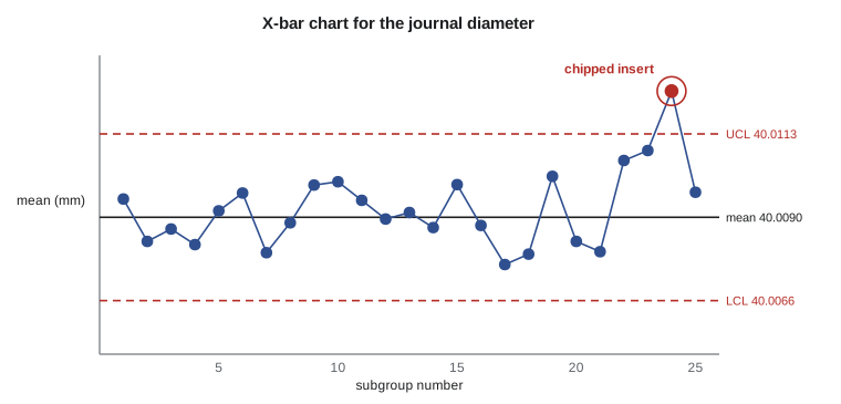
The most common chart for measured dimensions is the X-bar and R chart. At regular intervals, a small subgroup of consecutive parts, typically five, is measured. The subgroup mean \(\bar x\) and range \(R\) are plotted. After about 20 to 25 subgroups from a stable process, the grand mean \(\bar{\bar x}\) and average range \(\bar R\) give the center lines and control limits, using constants that depend on subgroup size (for \(n = 5\), \(A_2 = 0.577\), \(D_3 = 0\), \(D_4 = 2.114\), \(d_2 = 2.326\)).

A point outside the control limits signals a special cause. So do patterns: seven or more points in a row on one side of the center line, steady trends up or down, or cycles. Control limits describe what the process does; they are not tolerance limits, which describe what the customer needs. A process can be in control and still make parts out of tolerance if its natural spread is too wide.

Process capability

Capability indices compare the process spread with the tolerance. With upper and lower specification limits \(USL\) and \(LSL\), mean \(\mu\) and standard deviation \(\sigma\):

\(C_p\) measures potential capability if the process were perfectly centerd; \(C_{pk}\) accounts for where it actually sits. A value of 1.0 means the process just fits its ±3σ spread within the tolerance, giving about 2700 defective parts per million if the distribution is normal. Automotive and agricultural equipment customers commonly require \(C_{pk} \geq 1.33\) for ongoing production and 1.67 for new processes and safety-critical characteristics. Capability must be measured only after the process is shown to be in statistical control, because an unstable process has no single capability.

# X-bar and R chart and capability for the 40 mm journal (tolerance 40.000 to 40.016 mm)
import random, statistics

LSL, USL = 40.000, 40.016
A2, D3, D4, d2 = 0.577, 0.0, 2.114, 2.326          # constants for subgroups of 5

# Simulated study: 25 subgroups of 5 from a stable grinder (seeded so the output repeats)
random.seed(280)
subgroups = [[random.gauss(40.0091, 0.0018) for _ in range(5)] for _ in range(25)]
xbars = [statistics.mean(s) for s in subgroups]
ranges = [max(s) - min(s) for s in subgroups]
xbb, rbar = statistics.mean(xbars), statistics.mean(ranges)
print(f"Simulated study: grand mean {xbb:.4f} mm, average range {rbar:.4f} mm")
print(f"X-bar limits {xbb - A2*rbar:.4f} to {xbb + A2*rbar:.4f} mm; R chart UCL {D4*rbar:.4f} mm")
out = [i + 1 for i, x in enumerate(xbars) if not xbb - A2*rbar <= x <= xbb + A2*rbar]
print("Subgroups outside the X-bar limits:", out if out else "none")

def capability(mean, sigma):
    cp = (USL - LSL) / (6 * sigma)
    cpk = min(USL - mean, mean - LSL) / (3 * sigma)
    return cp, cpk

# Values reported in the launch study
mean, rbar_study = 40.0091, 0.0042
sigma = rbar_study / d2
for label, m in (("as run", mean), ("recenterd to 40.008", 40.008)):
    cp, cpk = capability(m, sigma)
    print(f"\n{label:20s}: sigma = {sigma*1000:.2f} um, Cp = {cp:.2f}, Cpk = {cpk:.2f}")

# Takt time for the KG-40 line
demand, days, minutes = 3000, 230, 450
takt = minutes / (demand / days)
print(f"\nTakt time: {takt:.1f} min per gearbox, {takt / 4:.1f} min per shaft (4 shafts per gearbox)")

# Overall equipment effectiveness of the shaft cell in its first month
A, P, Q = 0.86, 0.91, 0.985
print(f"OEE = {A:.2f} x {P:.2f} x {Q:.3f} = {A*P*Q:.1%}")

Simulated study: grand mean 40.0090 mm, average range 0.0040 mm
X-bar limits 40.0066 to 40.0113 mm; R chart UCL 0.0086 mm
Subgroups outside the X-bar limits: none

as run              : sigma = 1.81 um, Cp = 1.48, Cpk = 1.27

recenterd to 40.008 : sigma = 1.81 um, Cp = 1.48, Cpk = 1.48

Takt time: 34.5 min per gearbox, 8.6 min per shaft (4 shafts per gearbox)
OEE = 0.86 x 0.91 x 0.985 = 77.1%

Cost estimating

A manufacturing cost estimate builds up the cost of each part from its operations. For every step, the estimator determines the cycle time from the methods of this course, multiplies it by the hourly rate of the machine and labor, adds setup cost spread over the batch, adds material at its purchased cost plus scrap, and adds tooling amortized over the expected volume. Overhead, the cost of the building, supervision, engineering, quality and maintenance, is usually applied as a percentage of direct labor or machine cost, though activity-based costing assigns it more accurately to the products that cause it.

Estimates guide decisions throughout a product's life: choosing processes (Lesson 1), deciding whether to make or buy a part, quoting prices and finding where to focus improvement. For the KG-40, the estimate put the gearbox's manufacturing cost at 612 dollars, of which purchased bearings and seals are 21 percent, castings and forgings 24 percent, machining 31 percent, heat treatment 6 percent and assembly and test 18 percent. Machining is the biggest internal cost, which is why the shaft cell and tolerance review received so much attention.

Lean manufacturing

Lean manufacturing grew out of the Toyota Production System, which Taiichi Ohno and colleagues developed from the 1950s. Its central idea is to deliver exactly what the customer wants, when it is wanted, with the least waste. Lean thinking names seven classic wastes: overproduction, waiting, unnecessary transport, overprocessing, excess inventory, unnecessary motion and defects. Many practitioners add an eighth, unused human talent. Most factories, when first studied, find that a part spends well under 5 percent of its time in the plant actually being worked on; the rest is waiting, moving and sitting in inventory.

Lean tools attack these wastes. Value stream mapping draws every step of material and information flow for a product family, with times and inventories, to expose delays. Takt time, the available working time divided by customer demand, sets the pace production should match. Continuous flow and cells move parts one piece at a time between operations instead of in large batches. Pull systems such as kanban cards authorize production only when downstream processes use parts, preventing overproduction. Setup reduction, often called single-minute exchange of die, cuts changeover times so small batches become economic. Standardized work, 5S workplace organization, visual management, mistake-proofing devices (poka-yoke) and total productive maintenance stabilize processes so that flow is possible. Underlying all of it is kaizen, continuous improvement by the people who do the work.

Overall equipment effectiveness (OEE) multiplies a machine's availability (the share of planned time it actually runs), performance (its actual speed compared with its ideal speed) and quality (the share of good parts). World-class OEE for discrete manufacturing is often quoted around 85 percent; many plants find their first measurements between 40 and 60 percent, and the losses they uncover, breakdowns, long changeovers, minor stops, slow running and scrap, become the improvement agenda.

Six Sigma, developed at Motorola and popularized in the 1990s, complements lean with a structured, statistics-based method for reducing variation: define, measure, analyze, improve, control. Many companies combine the two as lean six sigma. The capability study above is a small example: measuring, finding that the process was off center, correcting it, and controlling it with a chart.

The KG-40 launch plan

The team's launch plan pulls the whole course together. Demand is 3000 gearboxes a year, about 13 per day over 230 working days, giving a takt time of about 35 minutes per gearbox on one eight-hour shift less breaks. Each gearbox needs four shafts, so the shaft cell has a takt of about 9 minutes per shaft, comfortably above its measured cycle time of 6.5 minutes, leaving capacity for growth. The housing is sand cast in gray iron by the supplier and machined on the horizontal machining center in two setups. Gear blanks are closed-die forged, hobbed, carburized and ground. The cradle is robot welded from low-carbon steel, now with a low-carbon forged lifting eye so no preheat is needed. The breather is injection molded in two cavities. Fixtures and gauges are printed in-house.

Every characteristic marked critical on the drawings has a control plan entry: how it is measured, how often, by what gauge, with what reaction if it goes out of control. Capability studies with Cpk of at least 1.67 are required at launch for the bearing journals, gear bores, housing bores and bolt torque. The assembly line records torques and test results against each serial number. A daily stand-up meeting at the line reviews OEE, scrap and any out-of-control signals, and an improvement board tracks actions. The plan is approved, and the first production gearboxes ship to the tractor plant the following month.