Introduction to power and refrigeration cycles

Every idea in this course comes together in the thermodynamic cycles that generate most of the world's electricity and provide most of its cooling. A steam power plant is a heat engine built from four steady-flow devices: a pump, a boiler, a turbine and a condenser. A refrigerator or heat pump is the same set of devices arranged to run the other way, with a compressor and an expansion valve. In this final lesson we analyze the ideal Rankine cycle, the model for steam power plants, then see how real plants depart from it and how cogeneration plants such as Northgate's use the same hardware more completely. We finish with the vapor-compression refrigeration cycle, which drives Northgate's chillers and its sewer heat pump.

Why not a Carnot cycle?

Lesson 10 showed that the Carnot cycle is the most efficient possible between two temperatures, so it is natural to ask why power plants do not use it. With steam, a Carnot cycle could run entirely under the dome: isothermal boiling, isentropic expansion, isothermal condensation, isentropic compression. Two practical problems kill it. The isentropic expansion would end at low quality, and water droplets erode turbine blades. Worse, the compression would have to handle a wet mixture of liquid and vapor, which no practical compressor or pump can do efficiently. The Rankine cycle, devised in the 1850s, fixes both problems: it superheats the steam before the turbine and condenses it completely before the pump.

The ideal Rankine cycle

The ideal Rankine cycle has four internally reversible processes. (1-2) Isentropic compression in a pump: saturated liquid from the condenser is pumped to boiler pressure. (2-3) Constant-pressure heat addition in the boiler: the compressed liquid is heated, boiled and superheated. (3-4) Isentropic expansion in a turbine, producing work. (4-1) Constant-pressure heat rejection in the condenser, which returns the fluid to saturated liquid. Each component is a steady-flow device, analyzed with the equations of Lesson 8.

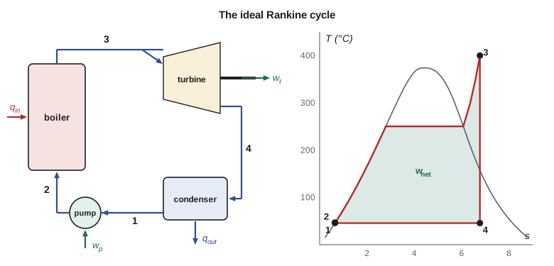
On a T-s diagram the cycle encloses an area equal to the net work, and the area under the heat-addition line equals \(q_{\text{in}}\). The steady-flow energy equation for each component, with negligible kinetic and potential energy changes, gives

Real cycles and how to improve them

Real pumps and turbines are not isentropic. With the isentropic efficiencies of Lesson 11, the turbine work falls and the pump work rises. Pressure drops in the boiler and piping, and heat losses, cut performance further. The program below repeats the ideal analysis and then applies efficiencies of 85 percent to both the turbine and the pump: the thermal efficiency drops from 35.3 to 30.0 percent.

# The Rankine cycle, cogeneration at Northgate, and a compression refrigeration cycle
# Steam properties: 10 kPa saturation and 4 MPa, 400 C, rounded from IAPWS-based tables
hf, hfg, sf, sfg, vf = 191.81, 2392.1, 0.6492, 7.4996, 0.001010   # 10 kPa
h3, s3 = 3214.5, 6.7714                                          # 4 MPa, 400 C
P_boiler, P_cond = 4000.0, 10.0

def rankine(eta_t=1.0, eta_p=1.0):
    h1 = hf
    wp = vf * (P_boiler - P_cond) / eta_p
    h2 = h1 + wp
    x4s = (s3 - sf) / sfg
    h4s = hf + x4s * hfg
    wt = eta_t * (h3 - h4s)
    h4 = h3 - wt
    qin, qout = h3 - h2, h4 - h1
    return wp, wt, qin, qout, (wt - wp) / qin, x4s, h4

for label, et, ep in (("ideal", 1.0, 1.0), ("actual (0.85, 0.85)", 0.85, 0.85)):
    wp, wt, qin, qout, eta, x4s, h4 = rankine(et, ep)
    print(f"{label:20s} wp = {wp:5.2f}  wt = {wt:7.1f}  qin = {qin:7.1f}  qout = {qout:7.1f}"
          f"  eta = {eta:.3f}")
print(f"isentropic turbine exit quality x4s = {rankine()[5]:.3f}; back work ratio = {rankine()[0] / rankine()[1]:.4f}")
print(f"Carnot limit between 400 C and 45.8 C: {1 - (45.81 + 273.15) / (400 + 273.15):.3f}")

# Cogeneration at Northgate: back-pressure turbine exhausting to the 1 MPa main
m, h_fw = 12.0, 445.1                       # kg/s; feedwater enthalpy after the pump
Q_boiler = m * (3214.5 - h_fw)
fuel = Q_boiler / 0.85                      # boiler efficiency 85 %
power = 3227 * 0.96                         # shaft power x generator efficiency
heat = (m - 0.48) * (2943.1 - 356.0) - 1000 # steam to buildings, less about 1 MW of losses
print(f"\nboiler {Q_boiler:.0f} kW, fuel {fuel:.0f} kW, power {power:.0f} kW, heat delivered {heat:.0f} kW")
print(f"utilization factor = {(power + heat) / fuel:.3f}")

# Ideal compression refrigeration cycle, R-134a, evaporating at -10 C and condensing at 40 C (rounded values)
h1, h2, h3r = 244.5, 278.0, 108.3
qL, w = h1 - h3r, h2 - h1
print(f"\nrefrigeration: qL = {qL:.1f} kJ/kg, w = {w:.1f} kJ/kg, COP_R = {qL / w:.2f}, COP_HP = {(qL + w) / w:.2f}")
print(f"Carnot COP_R between -10 C and 40 C = {263.15 / 50:.2f}")

ideal                wp =  4.03  wt =  1069.9  qin =  3018.7  qout =  1952.8  eta = 0.353
actual (0.85, 0.85)  wp =  4.74  wt =   909.4  qin =  3017.9  qout =  2113.2  eta = 0.300
isentropic turbine exit quality x4s = 0.816; back work ratio = 0.0038
Carnot limit between 400 C and 45.8 C: 0.526

boiler 33233 kW, fuel 39097 kW, power 3098 kW, heat delivered 28803 kW
utilization factor = 0.816

refrigeration: qL = 136.2 kJ/kg, w = 33.5 kJ/kg, COP_R = 4.07, COP_HP = 5.07
Carnot COP_R between -10 C and 40 C = 5.26

Three changes raise the efficiency of a Rankine plant, all by raising the average temperature at which heat is added or lowering the temperature at which it is rejected. Lowering the condenser pressure lowers the rejection temperature; large plants condense at 5 to 10 kPa, limited by the temperature of the cooling water. Superheating the steam to higher temperatures raises the average heat-addition temperature and also dries the turbine exhaust; modern plants reach 600 °C or more, limited by the creep strength of steels. Raising the boiler pressure raises the boiling temperature; supercritical plants operate above 22 MPa. Two further refinements, reheat (expanding in stages and reheating the steam between them) and regeneration (heating the feedwater with steam extracted from the turbine), are the subject of a later course on power cycles. Northgate's deaerator, heated with steam from the main, is a simple form of regenerative feedwater heating.

Cogeneration: using the rejected heat

Even the best power stations reject more than half their fuel energy to cooling water at temperatures too low to be useful. Cogeneration, or combined heat and power, places the heat rejection at a temperature useful to someone: the Northgate turbine exhausts at 1 MPa and about 250 °C, hot enough to heat forty buildings. The price is less electricity per kilogram of steam, since the turbine expands only to 1 MPa instead of 10 kPa. The reward is that almost all the fuel energy is used. The performance of a cogeneration plant is measured by its utilization factor, the useful output (electricity plus delivered heat) divided by the fuel energy input:

The vapor-compression refrigeration cycle

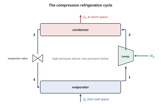
Reverse the Rankine cycle and replace the pump and turbine with a compressor and an expansion valve, and you have the vapor-compression refrigeration cycle, used in nearly every refrigerator, air conditioner, chiller and heat pump. The ideal cycle has four processes. (1-2) Saturated vapor from the evaporator is compressed isentropically to the condenser pressure, becoming superheated. (2-3) The vapor is cooled and condensed at constant pressure, rejecting heat \(q_H\) to the warm surroundings. (3-4) The saturated liquid is throttled through an expansion valve to the evaporator pressure, partly flashing to vapor and cooling sharply; this step is isenthalpic and irreversible, and is the one deliberate departure from a reversed Carnot cycle, accepted because an expansion turbine handling a wet mixture would recover little work at great cost. (4-1) The cold mixture evaporates at constant pressure, absorbing heat \(q_L\) from the cold space.

Refrigerant choice is now shaped by environmental rules as much as by thermodynamics. R-134a has no effect on stratospheric ozone but is a potent greenhouse gas, and the Kigali Amendment to the Montreal Protocol commits Canada, the United States and most other countries to phasing down such hydrofluorocarbons. New chillers and heat pumps increasingly use low-global-warming refrigerants such as hydrofluoroolefins, ammonia, carbon dioxide or hydrocarbons. Each has different properties, pressures and safety requirements, but the cycle analysis is identical: only the property tables change.

The course in one plant

Look back over the Northgate plant with the whole course in hand. The gauges on the morning round become absolute pressures (Lesson 1). Each energy flow is heat or work across a chosen boundary (Lesson 2). The steam's state is fixed by its phase and two properties (Lessons 3 and 4); combustion air, flue gas and instrument air are ideal gases (Lesson 5). Vessels and cylinders obey the closed-system first law (Lesson 6); the turbine, pumps, valves, deaerator and heat exchangers obey the steady-flow energy equation (Lessons 7 and 8); the air receiver charges as a transient (Lesson 9). The second law limits the turbine, the heat pump and any engine anyone offers to sell the plant (Lesson 10), and entropy shows where work potential is destroyed (Lesson 11). The cycles of this lesson tie them together. Further courses build on this base: power and refrigeration cycles in detail, gas mixtures and psychrometrics for air conditioning, combustion, heat transfer and fluid mechanics. Tomás finished his co-op term with a report recommending a larger heat pump and a lower loop temperature, every number in it traceable to the ideas in this course.