Laplace's equation, harmonic functions and the maximum principle

Laplace's equation \(\Delta u = 0\) is the equation of equilibrium: steady temperatures, electrostatic potentials, ideal fluid flow, the shape of a soap film stretched over a nearly flat wire frame. Its solutions, the harmonic functions, have a rigid and beautiful structure. Each value is the average of the values around it, so a harmonic function can have no peaks or pits inside its domain; its extreme values live on the boundary. This lesson proves the mean value property and the maximum principle, uses them to show that the Dirichlet problem has at most one solution and that it depends continuously on the boundary data, solves Laplace's equation on a rectangle by separation of variables, and computes solutions numerically by the iterative methods of Jacobi and Gauss–Seidel.

Harmonic functions

A function \(u\) with continuous second derivatives on an open set \(\Omega\) is harmonic there if \(\Delta u = 0\). In the plane, examples include \(1\), \(x\), \(y\), \(xy\), \(x^2 - y^2\), \(e^x\cos y\), \(e^x\sin y\) and \(\ln(x^2 + y^2)\) away from the origin. In polar coordinates, \(r^n\cos n\theta\) and \(r^n\sin n\theta\) are harmonic for every integer \(n\), as lesson 10 verifies. There is a deep connection with complex analysis: the real and imaginary parts of any analytic function \(F(z)\) of \(z = x + iy\) are harmonic, because the Cauchy–Riemann equations \(u_x = v_y\), \(u_y = -v_x\) give \(u_{xx} = v_{yx} = v_{xy} = -u_{yy}\). Thus \(z^2 = (x^2 - y^2) + 2ixy\) gives two harmonic functions, and \(z^n = r^ne^{in\theta}\) gives the polar family.

Harmonic functions form a vector space but not an algebra: sums and multiples are harmonic, but products usually are not, since \(\Delta(uv) = u\Delta v + v\Delta u + 2\nabla u\cdot\nabla v\). A harmonic function composed with a rotation, translation or scaling of the plane is still harmonic, reflecting the fact that the Laplacian is unchanged by rigid motions. This invariance is one reason Laplace's equation appears whenever a physical law has no preferred direction.

The mean value property

Let \(u\) be harmonic in a region containing the closed disc of radius \(R\) about a point \(\mathbf x_0\). Define the circular average

Differentiate under the integral sign: \(M'(r) = \frac{1}{2\pi}\int_0^{2\pi}\nabla u\cdot\mathbf e_\theta\,d\theta = \frac{1}{2\pi r}\oint_{|\mathbf x - \mathbf x_0| = r}\frac{\partial u}{\partial n}\,ds\). By the divergence theorem the flux integral equals \(\iint_{|\mathbf x - \mathbf x_0| < r}\Delta u\,dA = 0\). So \(M\) is constant, and since \(M(r) \to u(\mathbf x_0)\) as \(r \to 0\) by continuity,

Integrating over \(r\) gives the area version: \(u(\mathbf x_0)\) is also the average of \(u\) over the disc. Physically, in a steady temperature field each point is at the average temperature of any circle around it; any point hotter than its surroundings would be losing heat and could not be in equilibrium. The converse holds too: a continuous function with the mean value property is harmonic, and in fact infinitely differentiable. This is the source of the remarkable smoothness of harmonic functions.

The maximum principle

The strong maximum principle states that if \(u\) is harmonic on a connected open set \(\Omega\) and attains its maximum at an interior point, then \(u\) is constant. The proof uses the mean value property: if \(u(\mathbf x_0) = M\) is the maximum, the average of \(u\) over any small disc about \(\mathbf x_0\) equals \(M\) while no value exceeds \(M\), so \(u = M\) on the whole disc. The set where \(u = M\) is therefore open; it is also closed by continuity, and a nonempty set that is both open and closed in a connected set is everything.

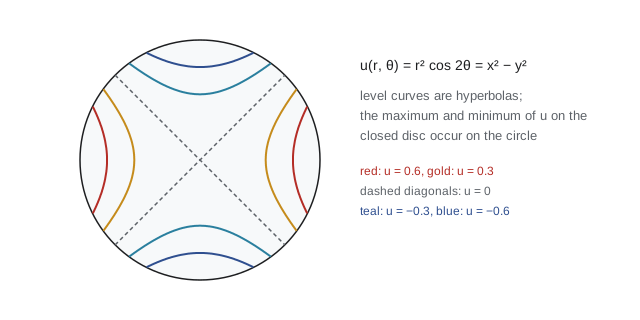
For a bounded region with boundary \(\partial\Omega\), the weak maximum principle is the version used most often: if \(u\) is harmonic in \(\Omega\) and continuous on its closure, then

A direct proof avoids the mean value property. Let \(v = u + \varepsilon|\mathbf x|^2\) for small \(\varepsilon > 0\). Then \(\Delta v = 4\varepsilon > 0\) in the plane. At an interior maximum of \(v\) the second derivatives \(v_{xx}\) and \(v_{yy}\) would both be non-positive, contradicting \(\Delta v > 0\). So \(v\) attains its maximum on the boundary, and \(u \le v \le \max_{\partial\Omega} u + \varepsilon\rho^2\), where \(\rho\) bounds \(|\mathbf x|\) on \(\Omega\). Letting \(\varepsilon \to 0\) proves the upper bound; applying it to \(-u\) gives the lower one.

Uniqueness and stability

The maximum principle settles the well-posedness questions of lesson 1 for the Dirichlet problem \(\Delta u = 0\) in \(\Omega\), \(u = g\) on \(\partial\Omega\). If \(u_1\) and \(u_2\) are two solutions with boundary data \(g_1\) and \(g_2\), their difference is harmonic with boundary data \(g_1 - g_2\), so

With equal data the solutions coincide, which is uniqueness. With nearly equal data they are uniformly close, which is continuous dependence. Errors in measuring the boundary temperature are never amplified inside. For the Neumann problem, with \(\partial u/\partial n = h\) prescribed, the divergence theorem gives the compatibility condition \(\oint h\,ds = \iint\Delta u\,dA = 0\): the net heat flux into a body in equilibrium must be zero, and solutions are unique only up to an additive constant.

Separation of variables on a rectangle

Consider the steady temperature in a plate \(0 < x < a\), \(0 < y < b\) whose bottom, left and right edges are held at 0 and whose top edge has temperature \(f(x)\). Seeking \(u = X(x)Y(y)\) gives \(X''/X = -Y''/Y = -\lambda\). The homogeneous conditions on the left and right edges make \(X\) the familiar eigenfunction \(\sin(n\pi x/a)\) with \(\lambda_n = (n\pi/a)^2\). Then \(Y'' = \lambda_nY\) with \(Y(0) = 0\), whose solution is \(\sinh(n\pi y/a)\), growing rather than oscillating. Superposition and the top boundary condition give

Writing the coefficient as a ratio of hyperbolic sines makes the factor equal to 1 on the top edge. Below the top, the factor \(\sinh(n\pi y/a)/\sinh(n\pi b/a) \approx e^{-n\pi(b - y)/a}\) decays rapidly with \(n\): fine details of the boundary data are felt only near the boundary, and the interior sees a smoothed version. If all four edges carry nonzero data, solve four such problems, one per edge, and add them.

Iterative solution on a grid

Replace the square by a grid of spacing \(h\) and the Laplacian by the five-point difference \(\big(u_{i+1,j} + u_{i-1,j} + u_{i,j+1} + u_{i,j-1} - 4u_{i,j}\big)/h^2\). The discrete Laplace equation says each interior value is the average of its four neighbors, a discrete mean value property, and the discrete maximum principle follows by the same argument as before. The equations form a large sparse linear system. Jacobi's method, published by Carl Gustav Jacobi in 1845, replaces every value by the average of its neighbors from the previous sweep. The Gauss–Seidel method uses each new value as soon as it is computed, which roughly halves the number of sweeps. Successive over-relaxation (SOR), introduced by David Young and Stanley Frankel around 1950, overshoots each Gauss–Seidel update by a factor \(\omega\) between 1 and 2, and with the optimal \(\omega \approx 2/(1 + \sin(\pi h))\) reduces the work from order \(N^2\) sweeps to order \(N\) on an \(N \times N\) grid.

import math

def series(x, y, N=99):
    return sum(400 / (n * math.pi) * math.sinh(n * math.pi * y) / math.sinh(n * math.pi) * math.sin(n * math.pi * x)
               for n in range(1, N + 1, 2))

def solve(M, method, omega=1.0, tol=1e-6):
    # unit square, M x M interior points, top edge 100, other edges 0
    u = [[0.0] * (M + 2) for _ in range(M + 2)]
    for i in range(M + 2):
        u[i][M + 1] = 100.0                      # u[i][j]: i along x, j along y
    u[0][M + 1] = u[M + 1][M + 1] = 50.0          # corners: average of the two edges
    sweeps = 0
    while True:
        sweeps += 1
        change = 0.0
        if method == "Jacobi":
            new = [row[:] for row in u]
            for i in range(1, M + 1):
                for j in range(1, M + 1):
                    new[i][j] = 0.25 * (u[i+1][j] + u[i-1][j] + u[i][j+1] + u[i][j-1])
                    change = max(change, abs(new[i][j] - u[i][j]))
            u = new
        else:
            for i in range(1, M + 1):
                for j in range(1, M + 1):
                    gs = 0.25 * (u[i+1][j] + u[i-1][j] + u[i][j+1] + u[i][j-1])
                    val = u[i][j] + omega * (gs - u[i][j])
                    change = max(change, abs(val - u[i][j]))
                    u[i][j] = val
        if change < tol:
            return u, sweeps

M = 19                                            # h = 1/20
h = 1 / (M + 1)
w_opt = 2 / (1 + math.sin(math.pi * h))
for name, w in (("Jacobi", 1.0), ("Gauss-Seidel", 1.0), ("SOR", w_opt)):
    u, k = solve(M, name if name == "Jacobi" else "GS", w)
    c = u[(M + 1) // 2][(M + 1) // 2]
    print(f"{name:12s} omega = {w:.3f}: {k:5d} sweeps, centre {c:.4f}")
print(f"series value at centre {series(0.5, 0.5):.4f}")

# compare with the series at a few points, and check the discrete maximum principle
for (i, j) in ((5, 5), (10, 15), (15, 18)):
    print(f"(x, y) = ({i * h:.2f}, {j * h:.2f}): grid {u[i][j]:8.4f}, series {series(i * h, j * h):8.4f}")
inner = [u[i][j] for i in range(1, M + 1) for j in range(1, M + 1)]
print(f"interior min {min(inner):.4f} > 0 and max {max(inner):.4f} < 100: maximum principle holds")
# mean value property of the exact solution on a circle about (0.5, 0.4)
avg = sum(series(0.5 + 0.3 * math.cos(2 * math.pi * k / 200), 0.4 + 0.3 * math.sin(2 * math.pi * k / 200)) for k in range(200)) / 200
print(f"average on circle r = 0.3 about (0.5, 0.4): {avg:.4f}, value at centre {series(0.5, 0.4):.4f}")

Jacobi       omega = 1.000:  1060 sweeps, center 24.9999
Gauss-Seidel omega = 1.000:   563 sweeps, center 25.0000
SOR          omega = 1.729:    72 sweeps, center 25.0000
series value at center 25.0000
(x, y) = (0.25, 0.25): grid   6.8132, series   6.7972
(x, y) = (0.50, 0.75): grid  53.9751, series  54.0529
(x, y) = (0.75, 0.90): grid  72.7026, series  72.8863
interior min 0.2744 > 0 and max 89.9252 < 100: maximum principle holds
average on circle r = 0.3 about (0.5, 0.4): 17.6531, value at center 17.6531

On this 19 by 19 interior grid, Gauss–Seidel needs about half as many sweeps as Jacobi, and SOR with the optimal factor needs fewer than a tenth as many. The grid value at the center is 25 as well, because the symmetry argument of the worked example applies equally to the discrete equations. Elsewhere grid and series differ in the first or second decimal place, the discretization error of the five-point formula, which is of order \(h^2\) away from the discontinuous corners. The circular average of the exact solution matches its central value, as the mean value property requires.

Beyond the plane

Everything in this lesson extends to three dimensions with spheres in place of circles. The fundamental solution becomes \(1/|\mathbf x|\), the potential of a point charge, rather than \(\ln|\mathbf x|\), and the mean value property, maximum principle, uniqueness and stability hold with the same proofs. Laplace's own interest was gravitational: outside the masses that produce it, the Newtonian potential is harmonic, and expanding it in spherical harmonics, the three-dimensional analog of \(r^n\cos n\theta\), was his tool for studying the shapes of planets. Today the same expansions describe the Earth's gravity field measured by satellites and the electron orbitals of atoms.