Finite difference methods and stability

Separation of variables needs simple geometry, constant coefficients and linear equations. Real problems, a turbine blade, a layered soil, a nonlinear reaction, rarely oblige. Numerical methods fill the gap. The finite difference method replaces derivatives by differences on a grid and the PDE by a system of algebraic equations, which a computer solves. The catch is stability: a perfectly consistent scheme can produce garbage that grows exponentially if the time step is too large. This lesson builds explicit and implicit schemes for the heat equation and the leapfrog scheme for the wave equation, analyses their accuracy and stability by the method of von Neumann, and states the Courant–Friedrichs–Lewy condition that every explicit scheme for waves must obey.

Difference quotients

On a grid \(x_j = j\,\Delta x\), Taylor's theorem gives \(u(x + h) = u + hu' + \frac{h^2}{2}u'' + \frac{h^3}{6}u''' + \frac{h^4}{24}u'''' + \cdots\). Combining expansions at \(x \pm h\) yields the standard approximations

The forward difference is first-order accurate; the centered differences are second order, meaning the error falls by a factor of four when \(h\) is halved. The leading error term is the truncation error. In practice it competes with rounding error, which grows as \(h\) shrinks because of cancellation in \(u_{j+1} - u_j\); the program in lesson 1 chose its step sizes with this trade-off in mind.

The explicit scheme for the heat equation

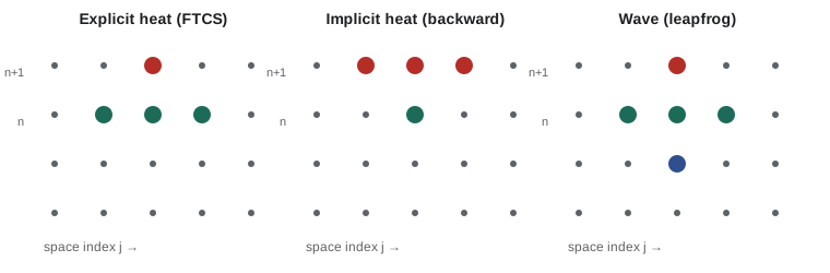
For \(u_t = \alpha u_{xx}\) on \(0 \le x \le L\), use a grid with \(\Delta x = L/J\) and time levels \(t_n = n\,\Delta t\), and write \(U_j^n\) for the approximation to \(u(x_j, t_n)\). A forward difference in time and a centered difference in space give the forward-time centered-space (FTCS) scheme

Each new value is computed directly from three old values, so the scheme is explicit and very cheap per step. Its truncation error is \(O(\Delta t) + O(\Delta x^2)\): substituting the exact solution leaves a residual of that size, so the scheme is consistent with the PDE. Boundary values are imposed directly at \(j = 0\) and \(j = J\) for Dirichlet conditions; a Neumann condition \(u_x = 0\) is handled with a ghost point, setting \(U_{-1} = U_1\).

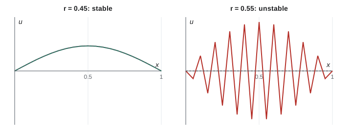
When \(r \le \frac12\), the coefficients \(r\), \(1 - 2r\) and \(r\) are all non-negative and sum to 1, so each new value is a weighted average of old ones. This gives a discrete maximum principle: the numerical solution never exceeds its initial and boundary maxima, and errors cannot grow. When \(r > \frac12\), the middle coefficient is negative and the averaging argument fails. The next section shows that the scheme then genuinely blows up.

Von Neumann stability analysis

John von Neumann's method, developed at Los Alamos in the 1940s and published by Crank and Nicolson in 1947 and by Charney, Fjørtoft and von Neumann in 1950, analyses how each Fourier mode is amplified per step. Substitute \(U_j^n = G^ne^{ik j\Delta x}\) into the scheme. The common factor cancels, leaving the amplification factor

Stability requires \(|G| \le 1\) for every wavenumber. Since \(\sin^2\) ranges over \([0, 1]\), \(G\) ranges over \([1 - 4r, 1]\), and \(|G| \le 1\) exactly when \(r \le \frac12\). For \(r > \frac12\), the shortest grid wave, with \(k\Delta x = \pi\) (alternating signs from point to point), has \(G = 1 - 4r < -1\): it flips sign and grows every step. Rounding errors contain this mode, so it appears and explodes even if the initial data are smooth. The stability limit \(\Delta t \le \Delta x^2/(2\alpha)\) is severe: halving \(\Delta x\) for accuracy forces four times as many time steps.

Compare with the exact solution: mode \(k\) decays by \(e^{-\alpha k^2\Delta t}\) per step. For small \(k\Delta x\), \(G \approx 1 - \alpha k^2\Delta t\), which matches. For high wavenumbers the scheme damps less accurately, but as long as \(|G| \le 1\), the error stays bounded. The Lax equivalence theorem of Peter Lax and Robert Richtmyer (1956) makes this precise: for a well-posed linear problem, a consistent scheme converges if and only if it is stable.

Implicit schemes and Crank–Nicolson

Evaluating the space difference at the new time level gives the backward Euler, or fully implicit, scheme \(-rU_{j-1}^{n+1} + (1 + 2r)U_j^{n+1} - rU_{j+1}^{n+1} = U_j^n\). Its amplification factor is \(G = 1/(1 + 4r\sin^2(k\Delta x/2))\), which lies in \((0, 1]\) for every \(r > 0\): the scheme is unconditionally stable. Each step requires solving a tridiagonal linear system, which the Thomas algorithm, a streamlined Gaussian elimination, does in about \(8J\) operations, so the cost per step is still proportional to the number of grid points. The accuracy is still only first order in time.

John Crank and Phyllis Nicolson, working on heat conduction problems, published in 1947 the scheme that averages the explicit and implicit space differences:

centered at the half step. Its truncation error is \(O(\Delta t^2) + O(\Delta x^2)\), and its amplification factor \(G = (1 - 2r\sin^2(k\Delta x/2))/(1 + 2r\sin^2(k\Delta x/2))\) satisfies \(|G| \le 1\) for all \(r\). It is the standard workhorse for diffusion problems. One caveat: for large \(r\), \(G \to -1\) for the highest modes, so sharp initial data produce slowly decaying oscillations; a few initial backward Euler steps, a remedy due to Rannacher, remove them.

The wave equation and the CFL condition

For \(u_{tt} = c^2u_{xx}\), centered differences in both variables give the leapfrog scheme

The first step uses the initial velocity: \(U_j^1 = U_j^0 + \Delta t\,g_j + \frac{\sigma^2}{2}\delta^2U_j^0\), which is second-order accurate. The von Neumann substitution gives \(G^2 - 2(1 - 2\sigma^2s^2)G + 1 = 0\) with \(s = \sin(k\Delta x/2)\). The two roots have product 1, so stability requires both to lie on the unit circle, which happens when \(|1 - 2\sigma^2s^2| \le 1\) for all \(s\), that is, when

This is the Courant–Friedrichs–Lewy condition, from the 1928 paper of Richard Courant, Kurt Friedrichs and Hans Lewy, which used difference equations to prove existence theorems for PDEs. Its meaning is geometric. The numerical solution at \((x_j, t_n)\) depends on grid data in \([x_j - n\Delta x, x_j + n\Delta x]\), its numerical domain of dependence. The true solution depends on data in \([x_j - ct_n, x_j + ct_n]\). If the numerical domain does not contain the true one, the scheme cannot possibly converge, because it never sees data that affect the answer. Requiring \(c\,\Delta t \le \Delta x\) is exactly this containment. Remarkably, for \(\sigma = 1\) the leapfrog scheme is exact for the one-dimensional wave equation: the update becomes \(U_j^{n+1} = U_{j+1}^n + U_{j-1}^n - U_j^{n-1}\), a discrete version of d'Alembert's formula.

Solvers in code

The program implements the explicit heat scheme at two values of \(r\) and compares with the exact series solution, then solves the same problem by Crank–Nicolson with large time steps using the Thomas algorithm, and finally runs the leapfrog scheme for a plucked string at Courant numbers 0.9, 1.0 and 1.05, checking the discrete energy.

import math

J = 20
dx = 1.0 / J
xs = [j * dx for j in range(J + 1)]
f = lambda x: math.sin(math.pi * x) + 0.5 * math.sin(3 * math.pi * x)
exact = lambda x, t: math.exp(-math.pi ** 2 * t) * math.sin(math.pi * x) + 0.5 * math.exp(-9 * math.pi ** 2 * t) * math.sin(3 * math.pi * x)

def ftcs(r, T):
    dt = r * dx * dx
    U = [f(x) + 1e-12 * (-1) ** j for j, x in enumerate(xs)]   # rounding-sized noise
    U[0] = U[-1] = 0.0
    steps = round(T / dt)
    for _ in range(steps):
        U = [0.0] + [U[j] + r * (U[j + 1] - 2 * U[j] + U[j - 1]) for j in range(1, J)] + [0.0]
    return U, steps * dt

def thomas(a, b, c, d):
    n = len(d); cp, dp = [0.0] * n, [0.0] * n
    cp[0], dp[0] = c[0] / b[0], d[0] / b[0]
    for i in range(1, n):
        m = b[i] - a[i] * cp[i - 1]
        cp[i] = c[i] / m if i < n - 1 else 0.0
        dp[i] = (d[i] - a[i] * dp[i - 1]) / m
    x = [0.0] * n; x[-1] = dp[-1]
    for i in range(n - 2, -1, -1):
        x[i] = dp[i] - cp[i] * x[i + 1]
    return x

def crank_nicolson(r, T):
    dt = r * dx * dx
    U = [f(x) for x in xs]; U[0] = U[-1] = 0.0
    n = J - 1
    a, b, c = [-r / 2] * n, [1 + r] * n, [-r / 2] * n
    steps = round(T / dt)
    for _ in range(steps):
        d = [r / 2 * U[j - 1] + (1 - r) * U[j] + r / 2 * U[j + 1] for j in range(1, J)]
        U = [0.0] + thomas(a, b, c, d) + [0.0]
    return U, steps * dt

for r in (0.45, 0.5, 0.55):
    U, t = ftcs(r, 0.3)
    err = max(abs(U[j] - exact(xs[j], t)) for j in range(J + 1))
    print(f"explicit r = {r:4.2f}: t = {t:.4f}, max error {err:.3e}")
for r in (0.5, 5.0, 20.0):
    U, t = crank_nicolson(r, 0.1)
    err = max(abs(U[j] - exact(xs[j], t)) for j in range(J + 1))
    print(f"Crank-Nicolson r = {r:4.1f}: {round(0.1 / (r * dx * dx)):4d} steps, max error {err:.3e}")

# leapfrog for a plucked string, c = 1, fixed ends, released from rest
p0 = lambda x: 0.02 * (x / 0.3 if x < 0.3 else (1 - x) / 0.7)
def leapfrog(sigma, T, N=50):
    h = 1.0 / N; dt = sigma * h; s2 = sigma * sigma
    X = [j * h for j in range(N + 1)]
    old = [p0(x) for x in X]
    cur = [0.0] + [old[j] + s2 / 2 * (old[j + 1] - 2 * old[j] + old[j - 1]) for j in range(1, N)] + [0.0]
    steps = round(T / dt)
    for _ in range(steps - 1):
        new = [0.0] + [2 * cur[j] - old[j] + s2 * (cur[j + 1] - 2 * cur[j] + cur[j - 1]) for j in range(1, N)] + [0.0]
        old, cur = cur, new
    # discrete energy at the half step between old and cur
    E = sum(0.5 * ((cur[j] - old[j]) / dt) ** 2 * h for j in range(N + 1)) + \
        sum(0.5 * (cur[j + 1] - cur[j]) * (old[j + 1] - old[j]) / h for j in range(N))
    return cur, X, E
for sigma in (0.9, 1.0, 1.05):
    U, X, E2 = leapfrog(sigma, 2.0)
    err = max(abs(U[j] - p0(X[j])) for j in range(len(X)))
    line = f"leapfrog sigma = {sigma:4.2f}: after one period max |U - initial| = {err:.3e}"
    if err < 1:
        E1 = leapfrog(sigma, 0.54)[2]
        line += f", discrete energy {E1:.6e} at t = 0.54 and {E2:.6e} at t = 2"
    print(line)
print(f"continuous energy of the initial shape {0.5 * 0.02 ** 2 * (1 / 0.3 + 1 / 0.7):.6e}")

explicit r = 0.45: t = 0.3004, max error 5.348e-04
explicit r = 0.50: t = 0.3000, max error 6.307e-04
explicit r = 0.55: t = 0.2998, max error 1.954e+04
Crank-Nicolson r =  0.5:   80 steps, max error 7.403e-04
Crank-Nicolson r =  5.0:    8 steps, max error 3.322e-04
Crank-Nicolson r = 20.0:    2 steps, max error 7.565e-02
leapfrog sigma = 0.90: after one period max |U - initial| = 6.848e-04, discrete energy 9.340136e-04 at t = 0.54 and 9.340136e-04 at t = 2
leapfrog sigma = 1.00: after one period max |U - initial| = 1.735e-17, discrete energy 9.297052e-04 at t = 0.54 and 9.297052e-04 at t = 2
leapfrog sigma = 1.05: after one period max |U - initial| = 6.985e+20
continuous energy of the initial shape 9.523810e-04

The initial data carry noise of size \(10^{-12}\) in the alternating mode, standing in for rounding error. The explicit scheme is accurate at \(r = 0.45\) and \(r = 0.5\) and destroyed at \(r = 0.55\), where that noise has been multiplied by nearly 1.2 at each of 218 steps. Crank–Nicolson stays accurate with time steps ten times larger than the explicit limit. With steps forty times larger it remains stable, but two steps are too few to follow the fast decay of the \(\sin 3\pi x\) mode, whose amplification factor is about \(-0.37\) per step instead of the true 0.012: unconditional stability is not unconditional accuracy. The leapfrog scheme returns the plucked string to its initial shape after one period exactly, to rounding, at \(\sigma = 1\), with a small dispersive error at \(\sigma = 0.9\), and blows up at \(\sigma = 1.05\). Its discrete energy, a grid version of \(\frac12\int(u_t^2 + c^2u_x^2)\), is the same at both times sampled; it differs slightly from the continuous energy because the grid cannot resolve the corner of the pluck.

Beyond one dimension

In two dimensions the explicit heat scheme on a square grid requires \(r \le \frac14\), and in three \(r \le \frac16\), so implicit methods become even more attractive; the alternating direction implicit method of Peaceman and Rachford (1955) solves only tridiagonal systems by treating one direction implicitly at a time. For waves the CFL condition becomes \(c\,\Delta t\sqrt{1/\Delta x^2 + 1/\Delta y^2} \le 1\). Complicated geometries are usually handled by finite element methods, which approximate the solution by piecewise polynomials on triangles or tetrahedra and grew out of structural engineering in the 1950s and 1960s. The stability ideas of this lesson, amplification factors, domains of dependence and the Lax equivalence theorem, carry over to all of them.