Boundary value problems in polar coordinates and Bessel functions

Rectangles suit Cartesian coordinates, but drums, pipes, cylindrical tanks, boreholes and the cross-section of a wire are round. On a disc, separation of variables works in polar coordinates, and two new things happen. The angular equation produces Fourier series in \(\theta\), with periodicity replacing boundary conditions. The radial equation, for Laplace's equation, has simple power solutions that lead to Poisson's integral formula; for the heat and wave equations it becomes Bessel's equation, whose solutions are the Bessel functions. Their zeros, which are not evenly spaced, are the reason a drum does not sound a clear musical pitch. This lesson develops both cases.

The Laplacian in polar coordinates

With \(x = r\cos\theta\), \(y = r\sin\theta\), the chain rule gives \(u_r = u_x\cos\theta + u_y\sin\theta\) and \(u_\theta = -u_xr\sin\theta + u_yr\cos\theta\). Differentiating once more and collecting terms, a careful but routine computation, yields

A quicker derivation uses the divergence form: the flux of \(\nabla u\) out of a thin polar sector, divided by its area, gives \(\frac1r(r\,u_r)_r + \frac{1}{r^2}u_{\theta\theta}\), which expands to the same thing. The coefficients \(1/r\) and \(1/r^2\) are singular at the origin, an artifact of the coordinates rather than of the solution; it will force us to discard solutions that blow up at \(r = 0\).

Laplace's equation on a disc

Seek harmonic functions on the disc \(r < a\) with boundary values \(u(a, \theta) = f(\theta)\). Put \(u = R(r)\Theta(\theta)\). Multiplying \(\Delta u = 0\) by \(r^2/(R\Theta)\) separates it:

The angle \(\theta\) and \(\theta + 2\pi\) describe the same point, so \(\Theta\) must be \(2\pi\)-periodic. The periodic solutions of \(\Theta'' + \lambda\Theta = 0\) are \(\Theta = 1\) for \(\lambda = 0\) and \(\cos n\theta\), \(\sin n\theta\) for \(\lambda = n^2\), \(n = 1, 2, \ldots\). The radial equation \(r^2R'' + rR' - n^2R = 0\) is an Euler equation, solved by \(R = r^m\) with \(m^2 = n^2\). So \(R = r^n\) or \(r^{-n}\) for \(n \ge 1\), and \(R = 1\) or \(\ln r\) for \(n = 0\). The solutions \(r^{-n}\) and \(\ln r\) are unbounded at the center, so for the disc we keep only

At \(r = a\) this is the Fourier series of \(f\), so \(a_n\) and \(b_n\) are its Fourier coefficients. The factor \((r/a)^n\) damps high harmonics in the interior, the same smoothing seen on the rectangle in lesson 9. At the center only \(a_0/2\) survives: the value at the center is the average of the boundary values, the mean value property again. For the region outside a disc, \(r > a\), the bounded solutions use \(r^{-n}\) instead; for an annulus \(a < r < b\) all four types, including \(\ln r\), are needed.

Poisson's integral formula

Substituting the coefficient formulas into the series and summing the geometric series \(\sum\rho^n\cos n\phi = \mathrm{Re}\,\frac{\rho e^{i\phi}}{1 - \rho e^{i\phi}}\) gives a closed form, found by Siméon Denis Poisson:

The Poisson kernel \(P = \frac{a^2 - r^2}{a^2 - 2ar\cos(\theta - \phi) + r^2}\) is positive, integrates to \(2\pi\) over \(\phi\), and as \(r \to a\) concentrates all its weight at \(\phi = \theta\). These properties show that \(u\) is a weighted average of the boundary values, which gives the maximum principle directly, and that \(u(r, \theta) \to f(\theta)\) as \(r \to a\) at every point where \(f\) is continuous, even if \(f\) is merely continuous with a Fourier series that diverges at some points. Poisson's formula thus solves the Dirichlet problem on the disc for every continuous boundary function.

Vibrations of a drum and Bessel's equation

Now consider a circular membrane of radius \(a\) clamped at its rim, governed by \(u_{tt} = c^2\Delta u\) with \(u(a, \theta, t) = 0\). Separating time first, \(u = V(r, \theta)\cos(\omega t)\) gives the Helmholtz equation \(\Delta V + k^2V = 0\) with \(k = \omega/c\). Separating \(V = R(r)\Theta(\theta)\) gives the same angular functions \(\cos n\theta\), \(\sin n\theta\) as before, and the radial equation

With \(s = kr\) this becomes Bessel's equation of order \(n\), \(s^2R'' + sR' + (s^2 - n^2)R = 0\). It was studied by Daniel Bernoulli in 1732 for the oscillations of a hanging chain and by Euler in 1764 for the drum, and Friedrich Wilhelm Bessel made a systematic study of it in 1824, in work on planetary perturbations. A power series solution by the method of Frobenius gives the Bessel function of the first kind,

The series converges for every \(s\), and \(J_n\) is bounded at the origin with \(J_0(0) = 1\) and \(J_n(0) = 0\) for \(n \ge 1\). A second independent solution, \(Y_n\), is unbounded at \(s = 0\) and must be excluded for a full disc, though it is needed for an annulus. For large \(s\), \(J_n(s) \approx \sqrt{2/(\pi s)}\cos(s - n\pi/2 - \pi/4)\): an oscillation like a cosine whose amplitude decays like \(s^{-1/2}\), because energy spreads out over circles of growing circumference.

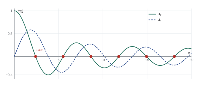
The boundary condition \(R(a) = J_n(ka) = 0\) requires \(ka\) to be a zero of \(J_n\). Writing \(j_{n,m}\) for the \(m\)-th positive zero, the allowed wavenumbers are \(k_{nm} = j_{n,m}/a\) and the frequencies are

The fundamental uses \(j_{0,1} \approx 2.405\). The next modes have frequency ratios \(j_{1,1}/j_{0,1} \approx 1.593\), \(j_{2,1}/j_{0,1} \approx 2.136\), \(j_{0,2}/j_{0,1} \approx 2.295\) and \(j_{3,1}/j_{0,1} \approx 2.653\). None of these is an integer, which is why a struck drum has an indistinct pitch, unlike a string with its harmonic series 1, 2, 3, and so on. Mode \((n, m)\) has \(n\) nodal diameters and \(m - 1\) nodal circles, patterns that Ernst Chladni made visible around 1787 by sprinkling sand on vibrating plates.

Fourier–Bessel series

To match an initial shape \(f(r)\) for the radially symmetric modes, we need to expand \(f\) in the functions \(J_0(j_{0,m}r/a)\). These are orthogonal with weight \(r\), a consequence of Sturm–Liouville theory for the radial equation \((rR')' + k^2rR = 0\):

so \(f(r) = \sum c_mJ_0(j_{0,m}r/a)\) with \(c_m = \frac{2}{a^2J_1(j_{0,m})^2}\int_0^a f(r)J_0(j_{0,m}r/a)\,r\,dr\). The weight \(r\) is the polar area element: the inner product is the ordinary integral over the disc. For \(f = 1\), the identity \(\int_0^s tJ_0(t)\,dt = sJ_1(s)\) gives \(c_m = 2/(j_{0,m}J_1(j_{0,m}))\). The same expansion solves heat flow in a long cylinder: a rod of radius \(a\) initially at \(T_0\), with surface held at 0, has \(u = T_0\sum c_mJ_0(j_{0,m}r/a)e^{-\alpha j_{0,m}^2t/a^2}\). The slowest decay rate is \(\alpha(2.405)^2/a^2 = 5.78\,\alpha/a^2\), compared with \(\pi^2\alpha/L^2\) for a slab of thickness \(L\).

Computing Bessel functions and the Poisson integral

The power series is exact in principle but suffers cancellation for large \(s\), where its terms grow enormous before alternating signs cancel them, so the program also uses Bessel's own integral representation \(J_n(s) = \frac1\pi\int_0^\pi\cos(n\tau - s\sin\tau)\,d\tau\), evaluated by the midpoint rule. It compares the two, finds the zeros of \(J_0\) by bisection, computes drum frequency ratios, checks the Fourier–Bessel coefficients of \(f = 1\), and evaluates Poisson's integral for the half-hot circle by the trapezoid rule, which is extremely accurate for smooth periodic integrands.

import math

def J_series(n, s, terms=60):
    tot, term = 0.0, (s / 2) ** n / math.factorial(n)
    for m in range(terms):
        tot += term
        term *= -(s / 2) ** 2 / ((m + 1) * (m + 1 + n))
    return tot

def J(n, s, M=256):
    # Bessel's integral (1/pi) * integral over [0, pi] of cos(n t - s sin t), by the midpoint rule
    return sum(math.cos(n * t - s * math.sin(t)) for t in [(k + 0.5) * math.pi / M for k in range(M)]) / M

for s in (1.0, 5.0, 12.0, 40.0):
    print(f"s = {s:4.1f}: series J0 = {J_series(0, s):+.10f}, integral J0 = {J(0, s):+.10f}")

def zeros(n, count):
    out, s, step = [], 0.5, 0.1
    while len(out) < count:
        if J(n, s) * J(n, s + step) < 0:
            lo, hi = s, s + step
            for _ in range(60):
                mid = (lo + hi) / 2
                lo, hi = (mid, hi) if J(n, lo) * J(n, mid) > 0 else (lo, mid)
            out.append((lo + hi) / 2)
        s += step
    return out

z0 = zeros(0, 6)
print("zeros of J0:", " ".join(f"{z:.4f}" for z in z0))
print("spacings:   ", " ".join(f"{b - a:.4f}" for a, b in zip(z0, z0[1:])), "(tend to pi)")
modes = sorted([(z, n, m + 1) for n in range(4) for m, z in enumerate(zeros(n, 3))])[:7]
print("drum frequency ratios:", ", ".join(f"({n},{m}) {z / z0[0]:.3f}" for z, n, m in modes))

# Fourier-Bessel coefficients of f = 1 on the unit disc, by Simpson's rule
def simpson(g, a, b, n=400):
    h = (b - a) / n
    return h / 3 * (g(a) + g(b) + sum((4 if i % 2 else 2) * g(a + i * h) for i in range(1, n)))
for z in z0[:3]:
    num = simpson(lambda r: J(0, z * r) * r, 0, 1)
    c = 2 * num / J(1, z) ** 2
    print(f"j = {z:.4f}: c = {c:+.5f}, formula 2/(j J1(j)) = {2 / (z * J(1, z)):+.5f}")
r = 0.3
print("partial sums of 1 at r = 0.3:", [round(sum(2 / (z * J(1, z)) * J(0, z * r) for z in zeros(0, K)), 4) for K in (1, 3, 10, 40)])

# Poisson integral for u = 1 on the upper half circle, 0 on the lower half
def poisson(r, th, M=4000):
    tot = 0.0
    for k in range(M):
        ph = (k + 0.5) * 2 * math.pi / M
        f = 1.0 if ph < math.pi else 0.0
        tot += (1 - r * r) / (1 - 2 * r * math.cos(th - ph) + r * r) * f
    return tot / M
for (rr, th) in ((0.0, 0.0), (0.5, math.pi / 2), (0.9, math.pi / 2), (0.5, 0.0), (0.7, -math.pi / 3)):
    exact = 0.5 + math.atan2(2 * rr * math.sin(th), 1 - rr * rr) / math.pi
    print(f"r = {rr}, theta = {th:+.3f}: Poisson {poisson(rr, th):.5f}, closed form {exact:.5f}")

s =  1.0: series J0 = +0.7651976866, integral J0 = +0.7651976866
s =  5.0: series J0 = -0.1775967713, integral J0 = -0.1775967713
s = 12.0: series J0 = +0.0476893108, integral J0 = +0.0476893108
s = 40.0: series J0 = -0.0901207900, integral J0 = +0.0073668906
zeros of J0: 2.4048 5.5201 8.6537 11.7915 14.9309 18.0711
spacings:    3.1153 3.1336 3.1378 3.1394 3.1401 (tend to pi)
drum frequency ratios: (0,1) 1.000, (1,1) 1.593, (2,1) 2.136, (0,2) 2.295, (3,1) 2.653, (1,2) 2.917, (2,2) 3.500
j = 2.4048: c = +1.60197, formula 2/(j J1(j)) = +1.60197
j = 5.5201: c = -1.06480, formula 2/(j J1(j)) = -1.06480
j = 8.6537: c = +0.85140, formula 2/(j J1(j)) = +0.85140
partial sums of 1 at r = 0.3: [1.4002, 0.8686, 1.0545, 0.9862]
r = 0.0, theta = +0.000: Poisson 0.50000, closed form 0.50000
r = 0.5, theta = +1.571: Poisson 0.79517, closed form 0.79517
r = 0.9, theta = +1.571: Poisson 0.96652, closed form 0.96652
r = 0.5, theta = +0.000: Poisson 0.50000, closed form 0.50000
r = 0.7, theta = -1.047: Poisson 0.12674, closed form 0.12674

The two formulas agree for small \(s\) while the series loses accuracy at \(s = 40\). The zeros of \(J_0\) agree with the figure and their spacings decrease toward \(\pi\), as the large-argument cosine approximation predicts. The overtone ratios confirm that the drum's spectrum is inharmonic. The Fourier–Bessel coefficients computed by quadrature match the closed form, and the partial sums at \(r = 0.3\) approach 1, though with the slow oscillating convergence expected from the jump in \(f\) at the rim. Poisson's integral agrees with the closed-form solution to five decimal places.