Why analysis: from calculus to proof

In calculus you learned to differentiate, integrate and sum series, and you learned rules that almost always work. Real analysis asks why they work, and exactly when. It takes the familiar objects of calculus, such as limits, continuity, derivatives and integrals, and rebuilds them from a small set of precise definitions about the real numbers. The payoff is twofold. First, you learn to tell the difference between a rule that is true and a rule that is merely usually true. Second, you gain the tools that the rest of modern mathematics, from probability to differential equations to numerical methods, is built on. This course assumes you can read and write proofs at the level of MATH-228 Introduction to Proofs: quantifiers, contradiction, induction, sets and functions.

Calculus works, but why?

Consider three statements you may have accepted in a first calculus course. A function that is continuous on a closed interval takes a largest value. A function whose derivative is zero everywhere on an interval is constant. If a sequence increases and never exceeds 10, it has a limit. Each statement sounds obvious, and each is true for the real numbers. But each is false for the rational numbers. The function \(f(x) = x^2 - 2\) is continuous on the rationals between 1 and 2, is negative at 1 and positive at 2, and yet it is never zero there, because \(\sqrt{2}\) is irrational. The increasing sequence of rational decimal approximations 1, 1.4, 1.41, 1.414, ... never exceeds 2 but has no rational limit.

So the familiar theorems of calculus depend on some property that the real numbers have and the rationals lack. That property is called completeness, and lesson 2 makes it precise. Much of this course consists of showing that one single axiom about the reals, the least upper bound property, is the hidden engine behind the intermediate value theorem, the extreme value theorem, the mean value theorem, the convergence of monotone sequences and the existence of the integral.

Some famous surprises

The history of analysis is full of plausible statements that turned out to be false. A few examples show why mathematicians in the nineteenth century decided they needed rigorous definitions.

• Rearranging a series can change its sum. The alternating harmonic series \(1 - \frac{1}{2} + \frac{1}{3} - \frac{1}{4} + \dots\) converges to \(\ln 2\), but by reordering its terms you can make it converge to any number you like. Bernhard Riemann proved this in the 1850s. Finite sums can be reordered freely; infinite sums cannot.

• A continuous function need not have a derivative anywhere. In 1872 Karl Weierstrass presented to the Berlin Academy a function that is continuous at every point and differentiable at none. Many earlier mathematicians had assumed that continuous functions are differentiable except at a few isolated points. Lesson 10 builds such a function.

• A limit of continuous functions need not be continuous. The functions \(f_n(x) = x^n\) on \([0, 1]\) are all continuous, but as \(n \to \infty\) they converge to a function that is 0 for \(x < 1\) and 1 at \(x = 1\). Augustin-Louis Cauchy stated in 1821 that such limits are always continuous, and the error was eventually traced to the difference between pointwise and uniform convergence, a topic for MATH-341 Real Analysis II.

• The derivative of a function can exist everywhere and still fail to be continuous. The function \(x^2 \sin(1/x)\), extended by 0 at the origin, is an example we will meet in lesson 10.

None of these surprises means calculus is wrong. They mean that the informal ideas of calculus, such as 'getting closer and closer' or 'no gaps in the graph', are too vague to decide hard cases. Analysis replaces them with definitions precise enough to be checked.

A short history

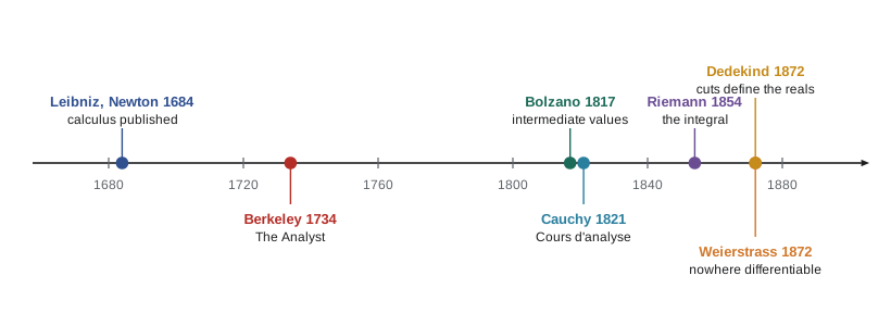
Isaac Newton and Gottfried Wilhelm Leibniz developed calculus in the late seventeenth century using infinitely small quantities. The method worked brilliantly, but its foundations were criticized; in 1734 Bishop George Berkeley mocked infinitesimals as 'the ghosts of departed quantities'. Through the eighteenth century, Leonhard Euler and others manipulated infinite series with great skill and occasional nonsense.

The rigorous approach began in the early nineteenth century. Bernard Bolzano, in Prague, gave in 1817 a proof of the intermediate value theorem based on what we now call the least upper bound property. Cauchy's textbook Cours d'analyze of 1821 defined limits, continuity and convergence in terms close to modern ones and introduced what we now call Cauchy sequences. Riemann defined the integral that bears his name in his 1854 habilitation thesis, published in 1868. Weierstrass, teaching in Berlin from the 1850s on, gave the epsilon-delta definitions their final form. Finally the real numbers themselves were constructed from the rationals: Richard Dedekind published his construction by cuts in 1872, and Georg Cantor gave a construction using Cauchy sequences in the same year. By the end of the century, calculus rested on the arithmetic of whole numbers and on set theory.

The epsilon game

The central idea of analysis is a way of making 'arbitrarily close' precise. Consider the claim that \(\frac{1}{n}\) gets close to 0 as \(n\) grows. What does that mean? One useful picture is a game between two players. A skeptic names a tolerance \(\varepsilon > 0\), as small as they like. You must respond with a threshold \(N\) such that every term past the threshold lies within \(\varepsilon\) of 0. If you can always respond, whatever \(\varepsilon\) the skeptic chooses, the limit is 0.

For \(\frac{1}{n}\), the response is easy: given \(\varepsilon\), pick any whole number \(N > \frac{1}{\varepsilon}\). Then for \(n \ge N\), \(\frac{1}{n} \le \frac{1}{N} < \varepsilon\). If the skeptic says \(\varepsilon = 0.001\), you answer \(N = 1001\). If they say \(\varepsilon = 10^{-9}\), you answer \(N = 10^9 + 1\). The definition of a limit in lesson 4 is exactly this game, written with quantifiers: \(\forall \varepsilon > 0 \; \exists N \; \forall n \ge N, \; |a_n - L| < \varepsilon\). The order of the quantifiers matters, as you saw in MATH-228: \(N\) may depend on \(\varepsilon\), but not the other way round.

The same game, with a tolerance on the output and a response on the input, defines the limit of a function and continuity. The definitions look forbidding at first, but they all say the same thing: the output can be made as close as you want to the target by making the input close enough.

from fractions import Fraction

def respond(eps):
    """Given a tolerance eps, return a threshold N with 1/n < eps for n >= N."""
    return int(1 / eps) + 1

for eps in [Fraction(1, 10), Fraction(1, 1000), Fraction(1, 10**6)]:
    N = respond(eps)
    worst = Fraction(1, N)          # the largest term from N on
    print(f"eps = {float(eps):g}:  N = {N},  1/N = {float(worst):.3g},  1/N < eps: {worst < eps}")

# The sceptic tries to find a term past N that is too far from 0.
eps = Fraction(1, 1000)
N = respond(eps)
bad = [n for n in range(N, N + 5000) if Fraction(1, n) >= eps]
print("terms past N that miss the tolerance:", bad)

eps = 0.1:  N = 11,  1/N = 0.0909,  1/N < eps: True
eps = 0.001:  N = 1001,  1/N = 0.000999,  1/N < eps: True
eps = 1e-06:  N = 1000001,  1/N = 1e-06,  1/N < eps: True
terms past N that miss the tolerance: []

What a proof in analysis looks like

Proofs in analysis have a characteristic shape. Here is a small example that we will prove properly in lesson 4 but can already read.

Claim. The sequence \(a_n = \frac{2n + 1}{n}\) converges to 2.

Scratch work. We want \(|a_n - 2| < \varepsilon\). Compute \(a_n - 2 = \frac{2n + 1 - 2n}{n} = \frac{1}{n}\). So we need \(\frac{1}{n} < \varepsilon\), that is, \(n > \frac{1}{\varepsilon}\).

Proof. Let \(\varepsilon > 0\). Choose a natural number \(N > \frac{1}{\varepsilon}\). For every \(n \ge N\) we have \(|a_n - 2| = \frac{1}{n} \le \frac{1}{N} < \varepsilon\). Hence \(a_n \to 2\). \(\blacksquare\)

There are two stages here. The scratch work runs backward from the goal to find a suitable \(N\). The proof runs forward: it starts with an arbitrary \(\varepsilon\), names \(N\), and verifies the inequality. The scratch work is not part of the proof and is usually not written down, but you cannot write the proof without it. Students often present only the scratch work, which shows that the goal follows from what you want, rather than that what you want follows from what you have.

Two features of this example are typical. First, the proof uses an inequality at the end, \(\frac{1}{n} \le \frac{1}{N}\), rather than an equation. Analysis is the art of estimation: we rarely compute exact values, but we bound errors. Second, the existence of a natural number larger than \(\frac{1}{\varepsilon}\) is itself a theorem about the real numbers, the Archimedean property, which we will prove from completeness in lesson 3.

Inequalities and the triangle inequality

Because analysis is about estimates, a few inequalities are used constantly. The most important is the triangle inequality: for all real \(x\) and \(y\),

\[|x + y| \le |x| + |y|.\]

Proof. We have \(-|x| \le x \le |x|\) and \(-|y| \le y \le |y|\). Adding gives \(-(|x| + |y|) \le x + y \le |x| + |y|\), which is the same as \(|x + y| \le |x| + |y|\). \(\blacksquare\)

Two consequences are used again and again. Replacing \(x\) by \(x - z\) and \(y\) by \(z - y\) gives \(|x - y| \le |x - z| + |z - y|\): the distance from \(x\) to \(y\) is at most the distance via any intermediate point \(z\). And the reverse triangle inequality says \(\big|\,|x| - |y|\,\big| \le |x - y|\): absolute values of nearby numbers are close.

A typical use: if \(|a - L| < \frac{\varepsilon}{2}\) and \(|b - M| < \frac{\varepsilon}{2}\), then \(|(a + b) - (L + M)| \le |a - L| + |b - M| < \varepsilon\). This 'epsilon over two' trick is how we will prove that the limit of a sum is the sum of the limits.

How this course is organized

The course moves in the same order as the subject developed logically, not historically.

• Lessons 2 and 3 set up the real numbers: the field and order axioms, the completeness axiom, suprema and infima, the Archimedean property and the density of the rationals.

• Lessons 4 to 6 study sequences: limits, the algebra of limits, monotone sequences, subsequences, the Bolzano–Weierstrass theorem, Cauchy sequences and series of real numbers.

• Lessons 7 to 9 study functions: limits, continuity, the intermediate value theorem, compactness, the extreme value theorem and uniform continuity.

• Lessons 10 and 11 study the derivative: the mean value theorem, its consequences, Taylor's theorem and L'Hôpital's rule.

• Lesson 12 defines the Riemann integral and proves the fundamental theorem of calculus.

Each lesson has worked proofs, common mistakes, a short Python experiment, a summary and practice problems with solutions. The Python code is never a substitute for proof. It is a laboratory: we use it to test conjectures, to see how fast sequences converge, and to find the right \(N\) or \(\delta\) before writing the proof that justifies it.

How to read analysis

Reading analysis is slower than reading most mathematics. A single line can carry a key estimate. Some habits help.

• Draw pictures. Most definitions have a picture: a band around a limit, a box around a point on a graph, a staircase of rectangles under a curve. This course provides many figures; draw your own too.

• Test definitions on examples and non-examples. Before trying to prove that a sequence converges, compute some terms. Before proving a function is continuous, sketch it.

• Track quantifiers. Most errors in analysis come from choosing \(N\) or \(\delta\) before \(\varepsilon\), or from letting a constant depend on a variable it should not depend on.

• Read proofs with a pencil. Check each inequality. Ask why each hypothesis is needed, and look for a counterexample when it is removed.

These habits are also the skills that employers and graduate programs look for in mathematics students: careful reasoning, precise writing, and the ability to tell a convincing argument from a plausible one.