
GEOM-499 · Lesson 7 of 12 · 20 min
Analysis
With both epochs processed, the team can finally ask the clients' questions of the data. Is the slope moving? Where, by how much and in which direction? Is the canal bank eroding? The analysis must answer these with numbers and uncertainties, separate real change from noise, and be honest about what the data cannot show. This lesson covers the four analyses at the heart of Coulee Watch: the stable-area check that tests whether the two epochs are truly comparable, the DEM of difference with its level of detection, the movement test for the slope targets, and the comparison with the radar velocities. It ends with canal cross-sections and with how the results are combined into findings.
First, check the two epochs agree where nothing changed
Before looking for change, the team looks for agreement. If the two terrain models are offset or tilted relative to each other, every difference will be contaminated. Nadia selects stable areas that should not have changed between October and April: the paved canal maintenance road, a concrete check structure, the gravel walkway on the crest and the tops of the control monuments. On these surfaces the difference between the epoch 2 and epoch 1 terrain models has a mean of 0.6 cm and a standard deviation of 3.9 cm, with no trend along or across the slope. A mean close to zero shows the two epochs share the same datum; a standard deviation of about 3.9 cm is consistent with the combined accuracy of the two models, which the next section uses.
If the mean had been several centimeters, the team would have looked for its cause, such as a control target misidentified in one epoch or a geoid model applied to one epoch only, before applying any correction. A blind shift to make stable areas agree would hide the cause and might be wrong elsewhere. Here no correction is needed.
The DEM of difference and the level of detection
A DEM of difference is computed by subtracting the epoch 1 terrain model from the epoch 2 model cell by cell. Negative values are loss of material, such as erosion; positive values are gain, such as deposition of material that has slumped from above. Each cell's difference is uncertain, so the team applies a threshold, the level of detection from lesson 2, calculated from the tested accuracy of each epoch. With RMSEz of 3.6 cm for epoch 1 and 3.4 cm for epoch 2, the threshold is about 9.7 cm. Cells whose absolute difference is below it are classed as no detectable change.
The script below runs this analysis on a 40 m by 12 m strip at the toe of the slope beside the canal, where the scans and the visual inspection both pointed to erosion. The real analysis runs over the whole site; the strip is used here because it shows the method in a few lines.
# Coulee Watch: DEM of difference between epochs and slope target movement
import math, random
random.seed(499)
nx, ny, cell = 40, 12, 1.0          # a 40 m x 12 m strip of the slope toe, 1 m cells
sig1, sig2 = 0.036, 0.034           # tested RMSEz of the two terrain models (m)
lod = 1.96 * math.sqrt(sig1 ** 2 + sig2 ** 2)
ero = dep = 0.0; cells_ero = cells_dep = 0
for j in range(ny):
    for i in range(nx):
        true = 0.0
        if 14 <= i <= 27 and j <= 5: true = -0.32 * math.exp(-((i - 20) / 6) ** 2)   # toe erosion
        if 30 <= i <= 37 and j >= 8: true = 0.15                                    # slumped debris
        d = true + random.gauss(0, math.sqrt(sig1 ** 2 + sig2 ** 2))
        if abs(d) < lod: continue
        if d < 0: ero += -d * cell * cell; cells_ero += 1
        else: dep += d * cell * cell; cells_dep += 1
print(f"level of detection {lod * 100:.1f} cm")
print(f"erosion {ero:6.1f} m3 in {cells_ero} cells, deposition {dep:5.1f} m3 in {cells_dep} cells")
print(f"net change {dep - ero:+6.1f} m3")
# total station targets: epoch 1 and 2 coordinates (m), sigma of each epoch 4 mm per axis
targets = {"T5": ((210.412, 85.207), (210.414, 85.205)),
           "T7": ((412.880, 61.330), (412.863, 61.318)),
           "T8": ((455.104, 58.902), (455.090, 58.892)),
           "T9": ((498.771, 60.115), (498.774, 60.111))}
s_d = math.sqrt(2) * 0.004
for k, ((x1, y1), (x2, y2)) in targets.items():
    d = math.hypot(x2 - x1, y2 - y1)
    az = math.degrees(math.atan2(x2 - x1, y2 - y1)) % 360
    flag = "significant" if d / s_d > 2.45 else "not significant"
print(f"{k} moved {d * 1000:4.1f} mm toward {az:5.1f} deg ({flag})")level of detection 9.7 cm erosion 18.7 m3 in 83 cells, deposition 4.8 m3 in 33 cells net change -13.9 m3 T5 moved 2.8 mm toward 135.0 deg (not significant) T7 moved 20.8 mm toward 234.8 deg (significant) T8 moved 17.2 mm toward 234.5 deg (significant) T9 moved 5.0 mm toward 143.1 deg (not significant)
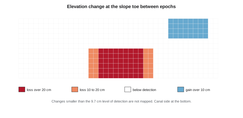
In the strip, about 18.7 cubic meters of material has been lost over 83 cells of one square meter each, concentrated in a scour about 14 m long where the canal bank meets the toe. About 4.8 cubic meters has been gained further along, where material appears to have slid down from above. The net change is a loss of about 14 cubic meters. Across the full 1.4 km reach the team finds two more, smaller areas of toe loss, both at bends in the canal where flow would be fastest.
Thresholding removes the noise, but it also hides real change smaller than the threshold. A slope that settles uniformly by 5 cm would be invisible in this map. The report therefore states the level of detection beside every volume and explains that the volumes are minimum estimates of detectable change, not a full sediment budget.
Worked problem
Volume from a DEM of difference
After thresholding, 120 cells of 0.5 m by 0.5 m show an average loss of 0.18 m. What volume of material was lost?
Show solution
- \[V = n \times A_\text{cell} \times \overline{\Delta z} = 120 \times 0.25 \times 0.18\]
- \[V = 5.4 \text{ m}^3\]
Answer: About 5.4 cubic meters. The volume depends on the threshold: if a less conservative 68 percent threshold were used, more cells would pass and the volume would be larger but less certain.
Testing whether the slope targets moved
The slope targets give precise movement at twelve points. For each target, the movement is the difference between its coordinates in the two epochs. Its uncertainty combines both epochs: with about 4 mm per axis in each epoch, the difference has about 5.7 mm per axis. In two dimensions a displacement is significant at 95 percent when it exceeds about 2.45 times that standard deviation, the 95 percent point of the distance distribution for two equal independent components, or about 14 mm.
The script shows four of the twelve targets. T7 and T8, on the middle row of the slope above the eroding toe, moved about 21 and 17 mm toward about 235 degrees, roughly southwest and downslope. Both movements are significant. T5 and T9 moved 3 and 5 mm in other directions, which is within noise. Of the full set of twelve, only T7 and T8 show significant movement. The vertical components, from the trigonometric heights, show T7 and T8 dropped by about 8 and 6 mm, which is consistent with a block sliding downslope and slightly rotating.
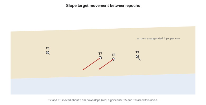
Movement at two adjacent targets in the same direction is much more persuasive than movement at one. The team checks the two targets' set-ups, the prism heights and the total station residuals in both epochs and finds no problem that could explain a 2 cm shift. It also checks that the control marks CW2 and CW4, from which the targets were observed, did not move: their positions in the two epochs' GNSS adjustments agree within 3 mm. The movement is real.
Comparing with the radar velocities
Liam extracts the descending-orbit persistent scatterer velocities around each target, averaging points within 30 m as planned. Near T7 and T8 the average line-of-sight velocity over the last three years is about −8 mm per year. Using the sensitivity from lesson 3, where the descending geometry sees about 81 percent of downslope motion, that corresponds to roughly 10 mm per year of downslope movement. Over the six months between epochs, that would be about 5 mm, much less than the 17 to 21 mm the targets measured.
The team does not hide the disagreement. Several explanations are possible: the radar points are mostly on the drier upper slope rather than right at the targets; the radar velocity is a three-year average and movement may have accelerated this year; the radar loses coherence during winter snow cover, so the winter months may be missing; and the target movement may include a seasonal component from freezing and thawing of the soil, which a slope at this latitude often shows. The report presents both measurements, explains the possible reasons for the difference and recommends that a geotechnical engineer review them together. The comparison was always designed to be indicative, and it has done its job by raising a question.
Canal cross-sections
For Marta, the most useful product is a set of canal cross-sections every 25 m along the reach, extracted from both terrain models and compared with the 1950s design section from the as-built drawings after converting them to the project datum. Most sections match the design within 10 to 15 cm, which reflects the original construction tolerance and sixty years of maintenance. Three sections near the slope toe show the bank set back by 40 to 70 cm from the design line and a bulge of slumped material on the upper bank. These coincide with the toe erosion area and with T7 and T8 above it.
| Station | Bank set back from design | Change between epochs | Comment |
|---|---|---|---|
| 0+600 | 0.18 m | Below detection | Normal for age of canal |
| 0+625 | 0.41 m | −0.12 m at toe | Start of erosion area |
| 0+650 | 0.68 m | −0.29 m at toe | Deepest scour; below T7 |
| 0+675 | 0.52 m | −0.21 m at toe | Below T8; slumped material on upper bank |
| 0+700 | 0.22 m | Below detection | End of erosion area |
From numbers to findings
The analysis ends by turning results into findings, each one a sentence the client can act on and each supported by evidence and an uncertainty. The team writes four. First, the slope crest below the new houses shows no detectable change in surface height and no significant movement at the upper targets over the six months. Second, a block of slope above canal stations 0+625 to 0+700 moved about 2 cm downslope over the winter, measured at two targets, and the radar archive shows slower movement in the same area over several years. Third, the canal toe below that block lost at least 19 cubic meters of material, with the bank now up to 0.7 m behind its design line. Fourth, the two processes are probably linked, but establishing the mechanism needs geotechnical and hydraulic assessment.
These findings are deliberately careful. They do not say the slope is safe or unsafe, or that the canal caused the movement. They say what was measured, how well, and what the data suggest should be investigated. That is the professional limit of a geomatics analysis, and staying inside it is what makes the findings credible.
Common mistakes
MistakeComputing change before checking that stable areas agree between epochs.
InsteadTest stable surfaces first; an offset between epochs contaminates every difference.
MistakeReporting raw volumes without a threshold.
InsteadApply a level of detection and state it beside every volume.
MistakeTreating a single target's movement as proof of a slide.
InsteadLook for consistent movement at neighboring targets and rule out set-up and control problems.
MistakeHiding disagreement between radar and ground measurements.
InsteadReport both, explain possible reasons and recommend further investigation.
Summary and key terms
- A stable-area check confirms the two epochs share the same datum before change is measured.
- A DEM of difference shows loss and gain; a 95 percent level of detection separates real change from noise.
- Thresholded volumes are minimum estimates and must be reported with their threshold.
- Target displacements are significant when they exceed about 2.45 times their standard deviation in two dimensions.
- Radar velocities and ground measurements may disagree for good reasons; both are reported and explained.
- Findings state what was measured, with uncertainty, and stop short of geotechnical interpretation.
- DEM of difference
- A raster of elevation change made by subtracting one terrain model from another.
- Stable area
- A surface assumed not to change between epochs, used to check their alignment.
- Significant movement
- A displacement larger than its uncertainty allows at a stated confidence.
- Cross-section
- A profile of the ground across a feature such as a canal, extracted at a given station.
- Finding
- A concise statement of a result, its evidence and its uncertainty, written for the client.
- Seasonal movement
- Movement that repeats with the seasons, such as frost heave and thaw settlement.
Practice problems
Work each problem on paper first, then reveal the answer to check.
Stable areas show a mean difference of +4 cm between epochs. What should the team do first?
Show answer
Look for the cause, such as a control or datum error, before considering any correction.
Two epochs have RMSEz of 3.0 and 4.0 cm. What is the 95 percent level of detection?
Show answer
1.96 × √(3.0² + 4.0²) = 9.8 cm.
A target moved 11 mm with σd = 5.7 mm. Is the movement significant at 95 percent?
Show answer
No: 11 / 5.7 = 1.93, below 2.45.
Why are thresholded volumes called minimum estimates?
Show answer
Real changes smaller than the threshold are excluded.
Give two reasons the radar velocity could be smaller than the target movement.
Show answer
Different locations, multi-year averaging, winter coherence loss, seasonal frost movement (any two).
Why does the team not say the slope is safe or unsafe?
Show answer
That is a geotechnical judgment outside the scope and competence of the geomatics analysis.
Lesson quiz · 5 questions
Score 60% or more to complete this lesson.
Create a free account to save your progress, take quizzes and earn a certificate.