
GEOM-499 · Lesson 3 of 12 · 22 min
Data sources and methods
With the requirements signed, the team has to decide how to meet them. Two questions come first. What data already exist that the project can use, and what must the team collect itself? And for the data it collects, which methods give the required accuracy over the required area within the time and equipment available? This lesson works through both questions for Coulee Watch, then sets out the method chosen for each requirement and the reasons for it. The choices matter beyond this project: a client paying for a monitoring program wants to know why each method was chosen and what it can and cannot see.
Start with what exists
A data search is cheap and often saves weeks. The team divides it into themes: elevation, imagery, geodetic control, property and infrastructure, radar satellite data and the client's own records. For each source Liam records the provider, the license, the date of capture, the datum and epoch, the stated accuracy and any restrictions. A source with an unknown datum or an unstated accuracy is not discarded, but it is marked as reference only and is never used to measure change.
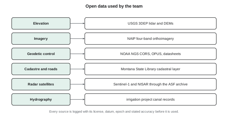
In Montana the useful sources include USGS 3D Elevation Program lidar and elevation models, NAIP orthoimagery flown in the growing season, the NOAA National Geodetic Survey's continuously operating reference stations, the OPUS processing service and published control datasheets, and the statewide cadastral layer from the Montana State Library. Radar data come from the European Sentinel-1 mission and from NISAR, whose data are distributed through NASA's Alaska Satellite Facility archive. Federal data are generally in the public domain, while state data come with their own terms of use.
The clients' records are just as important. The project has as-built drawings of the canal from the 1950s, a log of liner repairs and its own seepage observations. The city has the Coulee Ridge design files, the geotechnical report and the subdivision survey. Coulee Geomatics has its earlier lidar of the coulee banks from the laser scanning course and the radar velocity maps from the remote sensing and data science work. These give the project an epoch zero: earlier surveys that are not accurate enough to measure small change but that show the long-term shape of the slope and where it has moved before.
| Source | Use in Coulee Watch | Limitation |
|---|---|---|
| Public lidar elevation model | Context, planning flight heights, long-term change | Older epoch; about 10 cm accuracy; not for 10 cm change |
| Mentor firm's earlier lidar | Epoch zero for the steepest banks | Different sensor and datum realization; reference only |
| Public orthoimagery | Site planning, target sites, access routes | Coarser than required; leaf-on season |
| Continuously operating station CR1 | Datum tie for the new control network | Single station; needs a check against a second one |
| Radar satellite archive | Regional movement velocities since 2017 | Line of sight only; loses coherence on vegetation and snow |
| Canal as-built drawings | Design cross-section to compare with today | Old datum; scanned paper; uncertain |
Choosing methods for what must be collected
The methods the team could use span six orders of magnitude in area and two in accuracy. At one end, a total station measuring prisms on fixed targets gives millimeter-level positions but only at a few points. Static GNSS gives a few millimeters at a mark after hours of observation. A terrestrial laser scanner gives dense points with errors of several millimeters over a few hundred meters. Drone photogrammetry and mobile lidar cover square kilometers with errors of a few centimeters. Radar interferometry covers whole regions with millimeter sensitivity to motion, but only along one direction and only on ground that keeps a stable radar signature.
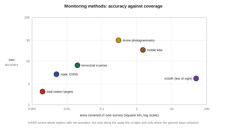
No single method answers both clients' questions. The team therefore designs a layered approach, a common pattern in monitoring. A sparse, very accurate layer of control and targets anchors everything else and measures movement at chosen points. A dense layer of drone photogrammetry and laser scanning maps the whole surface and its change. A regional layer of radar interferometry shows the pattern of movement around the site over several years and helps decide whether the measured points are representative.
Drone photogrammetry or lidar?
For the dense surface the team compares drone photogrammetry with drone lidar and with the terrestrial scanner. Photogrammetry produces an orthomosaic for free, uses equipment the university already owns and reaches about 2 to 4 cm vertically on bare, textured ground when control is good. Its weakness is vegetation: it reconstructs the top of the grass and shrubs, not the ground. Drone lidar penetrates gaps in vegetation and gives a better ground model under the shrubs on the lower slope, but the university does not own a lidar drone and renting one would use most of the cash budget.
The terrestrial scanner owned by Coulee Geomatics fills the gap. Ines Dahl agrees to lend it for two days in each epoch. Scanned from four stations at the foot of the slope, it gives millimeter-level points on the steep, eroding toe beside the canal, where the drone sees the surface at a low angle. The final choice is drone photogrammetry for the whole area, flown twice per epoch with nadir and oblique camera angles, plus terrestrial scans of the 300 m of toe where erosion is suspected.
Radar interferometry as a regional layer
Interferometric synthetic aperture radar compares the phase of radar echoes from repeated satellite passes. Persistent scatterer and small baseline techniques track the phase over many images to estimate a velocity at each stable point, often to a millimeter or two per year. The catch is the measuring direction. A radar satellite looks sideways from its orbit, so it measures only the component of movement along its line of sight. A slope that moves straight down toward the west is seen well by a satellite looking from the west, poorly by one looking from the east.
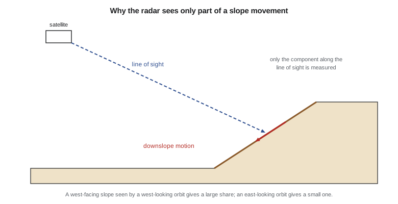
Liam computes how much of a downslope movement each orbit direction would see on the Coulee Watch slope, which faces west-southwest at about 24 degrees. The script builds a unit vector from the ground to the satellite for each geometry and a unit vector for motion straight down the slope, then takes their dot product.
# Coulee Watch: how much of a downslope movement does a radar satellite see?
import math
def unit_los(inc, head):
    """Ground-to-satellite unit vector (east, north, up) for a right-looking radar.
    inc = incidence angle, head = flight heading, both in degrees."""
    i, h = math.radians(inc), math.radians(head)
    look_az = h + math.pi / 2          # satellite looks to the right of its track
    return (-math.sin(i) * math.sin(look_az), -math.sin(i) * math.cos(look_az), math.cos(i))
def downslope(aspect, slope):
    """Unit vector of motion straight down a slope facing 'aspect' (deg from north)."""
    a, s = math.radians(aspect), math.radians(slope)
    return (math.sin(a) * math.cos(s), math.cos(a) * math.cos(s), -math.sin(s))
geom = {"ascending":  (39.0, 349.0), "descending": (39.0, 191.0)}
move = downslope(aspect=250.0, slope=24.0)      # the coulee face looks west-southwest
for name, (inc, head) in geom.items():
    u = unit_los(inc, head)
    seen = sum(a * b for a, b in zip(u, move))
    print(f"{name:10s} LOS sees {seen:+.2f} of the true downslope motion")
true = 12.0  # mm per year down the slope, a plausible slump rate
for name, (inc, head) in geom.items():
    u = unit_los(inc, head); seen = sum(a * b for a, b in zip(u, move))
print(f"{name:10s} {true:.0f} mm/yr downslope appears as {seen * true:+5.1f} mm/yr in line of sight")ascending LOS sees +0.25 of the true downslope motion descending LOS sees -0.81 of the true downslope motion ascending 12 mm/yr downslope appears as +3.0 mm/yr in line of sight descending 12 mm/yr downslope appears as -9.7 mm/yr in line of sight
The descending orbit, whose radar looks toward the west, sees about 81 percent of the motion as movement away from the satellite. The ascending orbit sees only about a quarter. This explains a puzzle from the earlier remote sensing work: the slump had shown clearly in descending data and hardly at all in ascending data. It also tells the team to use descending data for the velocity summary and to state in the report that the radar velocities are line-of-sight values that understate true slope motion.
Worked problem
Line-of-sight sensitivity
A slope moves 20 mm per year straight downslope. For the descending geometry the dot product of the line-of-sight unit vector and the downslope unit vector is −0.81. What velocity does the radar report, and what sign convention does it follow?
Show solution
- \[v_\text{LOS} = 20 \times (-0.81) = -16.2 \text{ mm/yr}\]
Answer: The radar reports about −16 mm per year. A negative value means the ground is moving away from the satellite, which for a west-facing slope seen from the west is consistent with downslope motion.
Methods for each requirement
| Requirement | Method | Why |
|---|---|---|
| R1 control | Static GNSS from CR1 plus a second station, digital leveling | Millimeter to centimeter accuracy, independent of the products it controls |
| R2 orthomosaic | Drone photogrammetry, 2.5 cm GSD | Covers the whole area quickly; university equipment |
| R3 terrain model | Drone photogrammetry plus terrestrial scans at the toe | Scans fill the steep toe the drone sees poorly |
| R4 change detection | Difference of epoch terrain models with level of detection | Uses the same products twice; uncertainty is computed |
| R5 slope targets | Total station sets from control marks | Millimeter-level horizontal movement |
| R6 radar summary | Descending persistent scatterer velocities | Regional context; best line-of-sight geometry |
Each method has a stated reason, and each reason can be checked. When the advisor asks why the team did not simply fly a drone lidar system, Sofia can point to the budget, to the toe scans that cover the vegetated part that matters most, and to the change detection requirement, which the photogrammetric terrain model can meet on open ground. A capstone examiner is looking for this kind of reasoning, not for the most expensive equipment.
Datums, epochs and a common frame
Data from many sources only combine if they share a reference frame. The team adopts one project frame for everything it collects: NAD83(2011) at epoch 2010.00, with NAVD 88 heights from the current hybrid geoid, projected on the project's low-distortion projection. Existing data are transformed into this frame, and the transformation is recorded. Because North America moves a few centimeters a year relative to the global frame, coordinates from precise point positioning or global products must be converted to the right epoch before they are compared. The geodesy courses showed how; here the team writes it into the method so nobody forgets.
Heights deserve special care. The drone software reports ellipsoidal heights from its onboard GNSS; the control network delivers orthometric heights; old canal drawings use a local datum. Mixing them would produce apparent changes of tens of meters or, worse, of a few centimeters that look like real erosion. The method statement therefore lists the height system of every input and the geoid model used to convert between them.
Writing the methods statement
The output of this stage is a two-page methods statement that the clients and the advisor approve. It lists the data sources and how each will be used, the methods chosen and the reasons, the reference frame, the equipment, the processing software and the tests that will show each requirement has been met. Writing it before the field work forces the team to discover gaps early. Liam finds one: nobody has planned how the radar velocities, which are given at scattered points, will be compared with the twelve slope targets. The team adds a step, using a buffer of 30 m around each target to average nearby radar points, and notes that the comparison is indicative only.
Common mistakes
MistakeUsing an old public elevation model to measure 10 cm of change.
InsteadUse existing data for context and long-term change only when its accuracy cannot support the requirement.
MistakeChoosing the most precise method for everything.
InsteadLayer methods: sparse precise points, dense surfaces, regional radar, each for its own purpose.
MistakeReporting radar line-of-sight velocity as slope movement.
InsteadState the geometry; line-of-sight values can understate or even hide downslope motion.
MistakeCombining data without recording datums, epochs and height systems.
InsteadFix one project frame and record every transformation into it.
Summary and key terms
- A data search records provider, license, date, datum, epoch and accuracy for every source.
- Existing data supply context and an epoch zero but may not be accurate enough to measure change.
- Methods trade accuracy against coverage; monitoring programs layer several methods.
- Drone photogrammetry maps open ground well; terrestrial scanning fills steep or vegetated areas.
- Radar interferometry measures only along the line of sight, so geometry decides what it can see.
- A single project reference frame, with recorded transformations and height systems, makes the data combinable.
- Epoch zero
- Earlier data used as a historical starting point rather than as a precise baseline.
- Layered monitoring
- Combining precise sparse methods, dense surface methods and regional methods in one program.
- Line of sight
- The direction from the ground to a radar satellite, along which interferometry measures movement.
- Persistent scatterer
- A point that keeps a stable radar signature over many images, used for velocity estimates.
- Methods statement
- A short document setting out the data, methods, frame, equipment and tests chosen for a project.
- Low-distortion projection
- A map projection designed so grid distances closely match ground distances over a project area.
Practice problems
Work each problem on paper first, then reveal the answer to check.
Why is the mentor firm's earlier lidar used only as reference?
Show answer
It was captured with a different sensor and datum realization and its accuracy does not support 10 cm change detection.
Which radar orbit suits a slope facing west-southwest, and why?
Show answer
The descending orbit, whose radar looks west, sees about 81 percent of the downslope motion.
Why are terrestrial scans added at the toe?
Show answer
The drone sees the steep toe at a low angle and the toe is where erosion is suspected.
What must happen to precise point positioning coordinates before comparison with the project frame?
Show answer
They must be transformed to the project datum and reference epoch.
What gap did writing the methods statement reveal?
Show answer
No plan to compare scattered radar velocities with the slope targets; a 30 m buffer average was added.
Name two things recorded for each data source.
Show answer
Any two of provider, license, capture date, datum and epoch, stated accuracy, restrictions.
Lesson quiz · 5 questions
Score 60% or more to complete this lesson.
Create a free account to save your progress, take quizzes and earn a certificate.