Data analysis with pandas and Matplotlib

NumPy arrays (Lesson 7) are ideal for grids of numbers of one type. Much engineering data is tabular in a richer way: each row a test specimen, a meter reading or a piece of equipment, and each column a different kind of value, some numbers, some text, some dates. The pandas library handles such tables, with labeled columns, mixed types, powerful grouping and summarizing, and built-in support for time series. Matplotlib turns the results into plots that people can understand. This lesson covers the DataFrame and Series, selecting and filtering, computed columns, grouping and summarizing, time series with resampling and rolling averages, missing data, and the principles and mechanics of making clear, honest plots. Together with NumPy, these tools let an engineer go from a raw export to a defensible conclusion in a few dozen lines.

DataFrames and Series

A pandas DataFrame is a table with labeled columns and an index labeling the rows. Each column is a Series, a one-dimensional labeled array, and columns can hold different types. DataFrames are usually created by reading a file, such as pd.read_csv("tests.csv"), pd.read_excel(...) or pd.read_json(...), or from a dictionary of lists, as in the example below. A few attributes and methods describe a new DataFrame quickly: .shape (rows and columns), .head() and .tail() (the first and last rows), .dtypes (the type of each column), .info() (types and missing values) and .describe() (summary statistics of numeric columns). Always look at a new dataset this way before analyzing it (Lesson 5).

Selecting, filtering and computing

df["col"] selects one column as a Series; df[["a", "b"]] selects several as a DataFrame. Rows are selected with a boolean mask, exactly as in NumPy: df[df["age_days"] == 28]. Masks combine with & and |, with each condition in parentheses. The .loc[rows, cols] indexer selects by labels and .iloc[rows, cols] by positions.

New columns are computed with whole-column arithmetic, which is vectorized: df["strength_MPa"] = df["load_kN"] * 1000 / area. Avoid looping over rows; it is slow and rarely necessary.

import math
import pandas as pd

tests = pd.DataFrame({
    "specimen": ["A1", "A2", "A3", "B1", "B2", "B3", "C1", "C2", "C3"],
    "mix":      ["A", "A", "A", "B", "B", "B", "C", "C", "C"],
    "age_days": [7, 28, 28, 7, 28, 28, 7, 28, 28],
    "load_kN":  [301, 482, 495, 265, 431, 446, 352, 571, 548],
})
area_mm2 = math.pi * 100 ** 2 / 4               # 100 mm diameter cylinders
tests["strength_MPa"] = tests["load_kN"] * 1000 / area_mm2     # new column, vectorized
print(tests.round(1).head(3))
print(tests["strength_MPa"].describe().round(1))
at28 = tests[tests["age_days"] == 28]             # filter rows
summary = at28.groupby("mix")["strength_MPa"].agg(["mean", "min", "count"]).round(1)
print(summary)
print("Mixes averaging at least 60 MPa at 28 days:", list(summary.index[summary["mean"] >= 60]))

  specimen mix  age_days  load_kN  strength_MPa
0       A1   A         7      301          38.3
1       A2   A        28      482          61.4
2       A3   A        28      495          63.0
count     9.0
mean     55.0
std      13.6
min      33.7
25%      44.8
50%      56.8
75%      63.0
max      72.7
Name: strength_MPa, dtype: float64
     mean   min  count
mix
A    62.2  61.4      2
B    55.8  54.9      2
C    71.2  69.8      2
Mixes averaging at least 60 MPa at 28 days: ['A', 'C']

Grouping and summarizing

The groupby method splits a table into groups by the values of one or more columns, applies a calculation to each group, and combines the results: "split, apply, combine". In the example, at28.groupby("mix")["strength_MPa"].agg(["mean", "min", "count"]) gives, for each concrete mix, the mean and lowest 28-day strength and the number of specimens, in one line. The same pattern answers many engineering questions: mean energy use by building and month, failure counts by equipment type, average travel time by route and hour.

Time series

Data indexed by time, such as meter readings, sensor logs, flows, temperatures and traffic counts, is where pandas excels. With a DatetimeIndex, a Series can be:

• Resampled to a different frequency: s.resample("D").sum() totals hourly kW into daily kWh, .mean() averages, .max() finds daily peaks.
• Smoothed with rolling windows: s.rolling(24).mean() is a 24-hour moving average.
• Filtered by time features: s[s.index.hour < 5] selects night hours; .dayofweek separates weekdays from weekends.
• Sliced by date: s["2026-01-12":"2026-01-18"] selects one week.

import numpy as np
import pandas as pd

t = pd.date_range("2026-01-05", periods=28 * 24, freq="h")        # four weeks, hourly
hour, dow = t.hour.to_numpy(), t.dayofweek.to_numpy()
occupied = (dow < 5) & (hour >= 7) & (hour < 19)                    # weekday working hours
rng = np.random.default_rng(42)
kW = 40 + 85 * occupied + 6 * rng.standard_normal(len(t))          # building electrical demand
s = pd.Series(kW, index=t, name="kW")

daily = s.resample("D").sum()                                       # kWh per day
print(daily.head(7).round(0))
print("Weekday mean:", round(daily[daily.index.dayofweek < 5].mean()), "kWh;",
      "weekend mean:", round(daily[daily.index.dayofweek >= 5].mean()), "kWh")
print("Peak demand:", round(s.max(), 1), "kW at", s.idxmax())
print("Night base load (0-5 h):", round(s[s.index.hour < 5].mean(), 1), "kW")
smooth = s.rolling(24).mean()                                       # 24-hour moving average
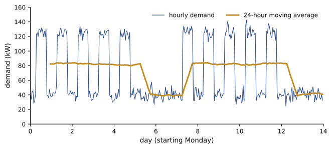
print("Highest 24-h average:", round(smooth.max(), 1), "kW")

2026-01-05    1977.0
2026-01-06    2006.0
2026-01-07    1967.0
2026-01-08    1957.0
2026-01-09    1950.0
2026-01-10     963.0
2026-01-11     947.0
Freq: D, Name: kW, dtype: float64
Weekday mean: 1975 kWh; weekend mean: 955 kWh
Peak demand: 142.4 kW at 2026-01-15 08:00:00
Night base load (0-5 h): 39.8 kW
Highest 24-h average: 84.6 kW

In a few lines, the analysis reveals the building's energy signature: about 1,975 kWh on weekdays and 955 kWh on weekends, a peak of 142 kW during working hours, and a base load of about 40 kW running all night and all weekend. That base load, nearly half the weekend energy, is often the first target in an energy audit: equipment, lighting and ventilation that run when nobody is there. The peak matters because many utilities charge large commercial customers for their highest demand in each billing period as well as for energy.

Missing data

Real tables have gaps. Pandas represents missing values as NaN (not a number) or NaT for times, and most calculations skip them by default: .mean() ignores NaN. That convenience can hide problems, so always count missing values first with df.isna().sum(). Then decide, by a rule stated in advance (Lesson 6), whether to drop rows (.dropna()), fill with a constant (.fillna(0)), carry the last value forward (.ffill()), or interpolate (.interpolate()). For sensor data, short gaps can often be interpolated; long gaps should be flagged rather than invented.

Making plots with Matplotlib

Matplotlib's object-oriented interface gives full control: fig, ax = plt.subplots() creates a figure and a set of axes; ax.plot, ax.scatter, ax.bar and ax.hist draw data; ax.set_xlabel, ax.set_ylabel, ax.set_title and ax.legend add labels; and fig.savefig("name.png", dpi=150) writes a file for a report. Several panels share a figure with plt.subplots(rows, cols). Pandas objects have a .plot() method that calls Matplotlib with sensible defaults, convenient for quick exploration.

import numpy as np
import matplotlib
matplotlib.use("Agg")                          # draw to a file, no window
import matplotlib.pyplot as plt

load = np.array([0, 5, 10, 15, 20, 25, 30])                       # kN
ext = np.array([0.000, 0.045, 0.089, 0.131, 0.178, 0.221, 0.264])  # mm
slope, icpt = np.polyfit(load, ext, 1)
resid = ext - (slope * load + icpt)

fig, (ax1, ax2) = plt.subplots(2, 1, figsize=(6, 6), sharex=True)
ax1.plot(load, ext, "o", label="measured")
ax1.plot(load, slope * load + icpt, "-", label=f"fit: {slope * 1000:.2f} um/kN")
ax1.set_ylabel("Extension (mm)")
ax1.set_title("Tensile test, 12 mm bar, 200 mm gauge length")
ax1.legend()
ax1.grid(alpha=0.3)
ax2.axhline(0, color="gray", lw=0.8)
ax2.plot(load, resid * 1000, "s")
ax2.set_xlabel("Load (kN)")
ax2.set_ylabel("Residual (um)")
fig.tight_layout()
fig.savefig("tensile.png", dpi=150)
print(f"Saved tensile.png; slope {slope * 1000:.2f} um/kN; largest residual {abs(resid).max() * 1000:.1f} um")

Saved tensile.png; slope 8.81 um/kN; largest residual 1.6 um

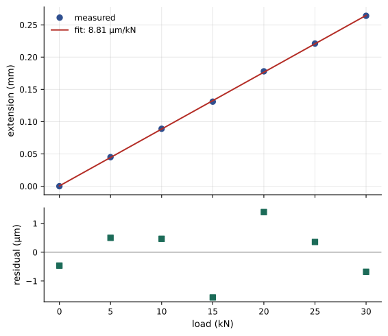
The residual panel is worth the extra lines. Residuals, the differences between data and fit, should scatter randomly around zero; a curved or trending pattern means the model is wrong (for example, a tensile test continued past the elastic limit), and a single large residual flags a possible bad reading. Here they are small and patternless, so the straight-line fit and the modulus calculated from it (Lesson 5) are trustworthy.

Plotting principles

The principles of ENGG-160 apply to every plot an engineer makes: choose the chart type to suit the message (line for trends over time, scatter for relationships, bars for comparisons, histograms for distributions); label axes with quantities and units; start bar charts at zero; avoid clutter; and make the main point visible, with an annotation if needed. A few Matplotlib-specific habits help:

• Use markers without lines for discrete measurements, and lines for continuous models or dense time series.
• Set figure sizes and font sizes for the final medium: a slide needs larger text than a report.
• Save as a vector format (SVG or PDF) for reports when possible, so lines stay sharp at any size, or as PNG at 150 to 300 dpi.
• Use a color-blind-friendly palette and distinguish series by marker or line style as well as color.
• Script every figure. A figure produced by code can be regenerated in seconds when data change or a reviewer asks for a different scale; a figure adjusted by hand cannot.

A reproducible analysis workflow

For any analysis that will support a decision, keep the raw data unchanged, do all cleaning and analysis in a script or notebook that runs from start to finish, and save outputs (tables and figures) from that script. Record the versions of key libraries and any assumptions or rules applied to the data. Then anyone, including you six months later, can rerun the analysis, check it and extend it. Lesson 12 returns to these practices.