NumPy in depth: arrays, broadcasting and linear algebra

Lesson 5 introduced NumPy arrays and whole-array arithmetic. Most engineering data, though, is not a single list of numbers: it is a table of readings from several sensors over time, a grid of temperatures over a plate, a matrix of stiffnesses, a set of design options evaluated under several load cases. NumPy's real power lies in multidimensional arrays and the rules that let operations combine arrays of different shapes without writing loops. This lesson covers array shapes and creation, indexing and slicing in two dimensions, boolean masks, broadcasting, aggregation along an axis, and the linear algebra routines that solve systems of equations and eigenvalue problems, with examples from strain gauges, beam selection, building energy and structural vibration.

Shapes and dimensions

Every NumPy array has a shape, a tuple giving its size along each dimension (axis). A list of 10 readings has shape (10,); a table of 3 gauges by 5 load steps has shape (3, 5); a temperature field on a 50 × 80 grid recorded at 100 times has shape (100, 50, 80). Arrays hold a single data type (dtype), usually 64-bit floats or integers, which is what makes them compact and fast.

Common ways to create arrays:

• np.array(list) from Python lists (nested lists for 2D).
• np.zeros((3, 5)), np.ones(...), np.full(shape, value) for arrays of a fixed value.
• np.arange(start, stop, step) for evenly spaced values by step, and np.linspace(a, b, n) for n evenly spaced values including both ends.
• np.eye(n) for an identity matrix, np.diag(v) for a diagonal matrix.
• np.loadtxt and np.genfromtxt to read numeric text files directly into arrays.

The reshape method changes the shape without changing the data (the total size must stay the same), .T transposes a 2D array, and .flatten() makes a 1D copy.

Indexing and slicing in two dimensions

For a 2D array A, A[i, j] is the element in row i and column j (counting from zero). Slices work on each axis: A[:, 2] is the whole of column 2, A[1, :] or simply A[1] is row 1, and A[0:2, 1:4] is a block. Negative indices count from the end. A slice of an array is a view of the same data, not a copy, so changing it changes the original; use .copy() when you need an independent array.

import numpy as np

# Strain readings: 3 gauges (rows) at 5 load steps (columns), microstrain
S = np.array([[ 0, 210, 405, 618, 822],
              [ 0, 198, 401, 597, 805],
              [ 0, 230, 455, 690, 931]])
print(S.shape, S.ndim, S.size, S.dtype)
print(S[1, 3])            # gauge 2, load step 4
print(S[:, -1])           # every gauge at the last step
print(S[2, 1:4])          # gauge 3, steps 2 to 4
high = S > 800
print(high.sum(), "readings above 800")
print(np.where(S > 800, "HIGH", "ok"))
print(S.T.shape, S.reshape(5, 3).shape, S.flatten()[:6])

(3, 5) 2 15 int64
597
[822 805 931]
[230 455 690]
3 readings above 800
[['ok' 'ok' 'ok' 'ok' 'HIGH']
 ['ok' 'ok' 'ok' 'ok' 'HIGH']
 ['ok' 'ok' 'ok' 'ok' 'HIGH']]
(5, 3) (5, 3) [  0 210 405 618 822   0]

A comparison such as S > 800 produces a boolean array of the same shape, a mask. Masks select elements (S[S > 800]), count them (mask.sum(), since True counts as 1), and combine with & (and), | (or) and ~ (not); note that each condition must be in parentheses, as in (S > 200) & (S < 600). The function np.where(condition, a, b) builds a new array taking a where the condition is true and b where it is false, a vectorized if-else.

Broadcasting

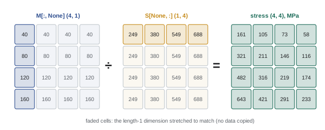
Arithmetic between arrays of different shapes follows the broadcasting rules: NumPy compares shapes from the last dimension backward, and two dimensions are compatible if they are equal or one of them is 1. A dimension of length 1 is stretched (without copying data) to match the other. So an array of shape (4, 1) combined with one of shape (1, 4) produces a (4, 4) result: every element of the first paired with every element of the second.

Broadcasting replaces nested loops with a single expression. Adding None as an index (or using reshape) inserts a dimension of length 1: M[:, None] turns a 1D array of 4 moments into a column of shape (4, 1).

import numpy as np

M = np.array([40, 80, 120, 160])                  # factored moments, kN m
names = ["W200x27", "W250x33", "W310x39", "W360x45"]
S = np.array([249, 380, 549, 688]) * 1e3          # section moduli, mm3
Fy, phi = 345.0, 0.9                              # yield stress MPa, resistance factor

# Broadcasting: a column of moments against a row of sections gives a 4 x 4 table
stress = (M[:, None] * 1e6) / S[None, :]          # MPa
ok = stress <= phi * Fy
print(np.round(stress).astype(int))
for i, m in enumerate(M):
    j = np.argmax(ok[i])                          # first True: lightest adequate section
    choice = names[j] if ok[i].any() else "none"
    print(f"M = {m:3d} kN m: lightest section {choice}")

[[161 105  73  58]
 [321 211 146 116]
 [482 316 219 174]
 [643 421 291 233]]
M =  40 kN m: lightest section W200x27
M =  80 kN m: lightest section W250x33
M = 120 kN m: lightest section W310x39
M = 160 kN m: lightest section W310x39

The 4 × 4 table of stresses comes from one line, M[:, None] / S[None, :], replacing two nested loops. Comparing it with the factored resistance φF_y gives a boolean table, and np.argmax on each row finds the first True, the lightest section that works, because the sections are listed in order of weight. A beam with a factored moment of 160 kN·m needs at least a W310×39 under these simplified assumptions (ENGG-130, Lesson 11, shows where the section modulus comes from). Real member selection also checks shear, deflection and lateral-torsional buckling.

Aggregating along an axis

Functions such as sum, mean, max, min, std and argmax reduce an array to fewer numbers. With no argument they reduce the whole array; with axis=0 they reduce down the rows, giving one result per column, and with axis=1 across the columns, giving one result per row. Remembering which is which is easier if you think of the axis as the one that disappears: a (7, 24) table reduced along axis=1 gives 7 values.

import numpy as np

days, hours = 7, 24
h = np.arange(hours)
day_mean = np.array([-4.0, -2.5, 1.0, 3.5, 2.0, -1.0, -6.0])      # daily mean temperature, C
swing = np.array([5.0, 6.0, 4.0, 7.0, 3.0, 5.5, 8.0])            # half the daily range, C
# 7 x 24 table: each row a day; broadcasting combines the day columns with the hour row
T = day_mean[:, None] + swing[:, None] * np.sin(2 * np.pi * (h[None, :] - 9) / 24)
print(T.shape)
print("Daily max:", np.round(T.max(axis=1), 1))
print("Daily min:", np.round(T.min(axis=1), 1))
print("Hourly mean over the week (first 6 h):", np.round(T.mean(axis=0)[:6], 1))
hdd = np.clip(18 - T, 0, None).sum() / 24        # heating degree-days from hourly data
print(f"Heating degree-days this week: {hdd:.1f}")
print("Hours below freezing:", int((T < 0).sum()), "of", T.size)

(7, 24)
Daily max: [ 1.   3.5  5.  10.5  5.   4.5  2. ]
Daily min: [ -9.   -8.5  -3.   -3.5  -1.   -6.5 -14. ]
Hourly mean over the week (first 6 h): [-4.9 -5.8 -6.3 -6.5 -6.3 -5.8]
Heating degree-days this week: 133.0
Hours below freezing: 91 of 168

The example builds a whole week of hourly temperatures from two short arrays by broadcasting, then summarizes it per day (axis=1) and per hour of the day (axis=0). Heating degree-days, a standard measure of heating demand used to estimate building energy use, are computed in one line with np.clip, which replaces values below zero by zero, so that only the hours colder than 18 °C count. Each operation that would need a loop over 168 values in plain Python is a single expression in NumPy.

Linear algebra

Many engineering problems lead to systems of linear equations Ax = b: mesh and nodal analysis of circuits (PHYS-131), forces in statically determinate trusses (ENGG-130), heat conduction on a grid, and the stiffness equations of structural analysis. Lesson 5 used np.linalg.solve for a small system. The same function solves systems with thousands of unknowns, using LU factorization (MATH-125), and you should use it rather than computing an inverse: np.linalg.inv(A) @ b is slower and less accurate.

The @ operator performs matrix multiplication (A @ B), while * multiplies element by element. Other useful routines include np.linalg.det (determinant), np.linalg.norm (vector and matrix norms), np.linalg.cond (condition number, which warns when a system is nearly singular and its solution sensitive to small errors), and np.linalg.eig and eigh for eigenvalues and eigenvectors.

import numpy as np

# Two-level frame: floor masses (kg) and level stiffnesses (N/m)
m1, m2 = 20000.0, 15000.0
k1, k2 = 4.0e7, 3.0e7
M = np.diag([m1, m2])
K = np.array([[k1 + k2, -k2],
              [-k2,      k2]])
# Natural frequencies: symmetric form A = M^(-1/2) K M^(-1/2), solved with eigh
Mh = np.diag(1 / np.sqrt(np.diag(M)))
w2, phi = np.linalg.eigh(Mh @ K @ Mh)             # eigenvalues in ascending order
modes = Mh @ phi
f = np.sqrt(w2) / (2 * np.pi)
print("Natural frequencies (Hz):", np.round(f, 2))
for i in range(2):
    v = modes[:, i] / modes[np.argmax(np.abs(modes[:, i])), i]
    print(f"Mode {i + 1} shape (floor 1, floor 2):", np.round(v, 3))

# Static check: lateral loads of 50 and 80 kN at the two floors
F = np.array([50e3, 80e3])
x = np.linalg.solve(K, F)
print("Floor displacements (mm):", np.round(x * 1000, 2))

Natural frequencies (Hz): [ 4.67 10.84]
Mode 1 shape (floor 1, floor 2): [0.569 1.   ]
Mode 2 shape (floor 1, floor 2): [ 1.    -0.758]
Floor displacements (mm): [3.25 5.92]

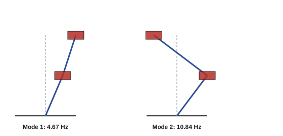
The two-story frame is modeled with floor masses and story stiffnesses. Its natural frequencies come from the eigenvalue problem Kφ = ω²Mφ: the first mode, at 4.67 Hz, has both floors moving the same way, the upper one more; the second, at 10.84 Hz, has them moving in opposite directions. Transforming to a symmetric matrix and using eigh guarantees real eigenvalues returned in ascending order. Engineers compare such frequencies with those of earthquakes, wind gusts, footfall or machinery to avoid resonance (PHYS-130). The static solve gives the floor displacements under lateral loads, 3.25 and 5.92 mm. Structural analysis programs solve exactly these equations, with thousands of degrees of freedom.

Random numbers

np.random.default_rng(seed) creates a random number generator; rng.normal(mean, sd, size), rng.uniform(a, b, size) and rng.integers(...) draw arrays of random values. Fixing the seed makes results reproducible, which is essential when a simulation is part of a report. Lesson 11 uses random arrays for Monte Carlo simulation of uncertain loads and reliability.

Performance habits

A few habits make NumPy code fast and correct:

• Avoid Python loops over array elements; look for a vectorized expression, a ufunc (np.sqrt, np.exp, np.maximum) or an aggregate.
• Preallocate arrays with np.zeros if you must fill them in a loop, rather than appending to a list and converting.
• Watch dtypes: integer arrays do integer arithmetic and can overflow silently for very large values; use floats for physical quantities.
• Check shapes with .shape whenever an operation surprises you; most NumPy bugs are shape mismatches that broadcasting quietly accepted.
• Remember that slices are views: modify a .copy() if the original must be preserved.