Algorithms, recursion and efficiency

Lesson 1 defined an algorithm as a precise, finite sequence of steps that solves a problem. For small problems almost any correct algorithm will do. As data grows, from a hundred readings to a hundred million, or from a ten-node network to a city's water system, the choice of algorithm can make the difference between an answer in a second and one that would take years. This lesson introduces the ideas computer scientists use to reason about algorithms: counting how work grows with problem size (big-O notation), searching and sorting, recursion for problems with a nested structure, and graph algorithms such as Dijkstra's shortest path, which route traffic, plan pipe networks and schedule projects. The goal is not to write your own versions of library routines, but to understand what they do, choose well among them, and recognize when a program will not scale.

Measuring efficiency

Timing a program on one computer tells you how long that run took, but not how the time will grow with more data. Computer scientists instead count the basic operations an algorithm performs as a function of the input size n, and describe the growth rate with big-O notation, keeping only the dominant term and ignoring constant factors:

• O(1): constant time, independent of n, such as looking up a dictionary key or an array element by index.
• O(log n): logarithmic, such as binary search, which halves the problem at each step.
• O(n): linear, such as summing a list or a linear search.
• O(n log n): typical of good sorting algorithms.
• O(n²): quadratic, such as comparing every item with every other, or nested loops over the same data.
• O(2ⁿ): exponential, such as trying every subset of n items; hopeless beyond a few dozen items.

import math

print("     n        log2 n         n log2 n             n^2")
for n in [10, 1_000, 100_000, 10_000_000]:
    print(f"{n:10,d} {math.log2(n):10.1f} {n * math.log2(n):18,.0f} {n ** 2:18,.0f}")

# Sorting with a key: work orders by priority, then by age
orders = [("WO-17", 2, 12), ("WO-03", 1, 40), ("WO-22", 3, 2), ("WO-09", 1, 5), ("WO-14", 2, 30)]
by_priority = sorted(orders, key=lambda o: (o[1], -o[2]))     # priority 1 first, oldest first
for wo, pri, age in by_priority:
    print(f"{wo}  priority {pri}  open {age:2d} days")

     n        log2 n         n log2 n             n^2
        10        3.3                 33                100
     1,000       10.0              9,966          1,000,000
   100,000       16.6          1,660,964     10,000,000,000
10,000,000       23.3        232,534,967 100,000,000,000,000
WO-03  priority 1  open 40 days
WO-09  priority 1  open  5 days
WO-14  priority 2  open 30 days
WO-17  priority 2  open 12 days
WO-22  priority 3  open  2 days

The table shows why growth rates matter more than raw speed. For ten items, all are trivial. For ten million, an O(n log n) algorithm needs about 230 million operations, a fraction of a second, while an O(n²) one needs 10¹⁴, roughly a day or more even on a fast computer. Nested loops that compare every reading with every other, harmless in testing with a few hundred values, are a common reason engineering scripts grind to a halt on real datasets.

Searching

Finding an item in an unsorted list requires checking items one by one, a linear search, O(n). If the list is sorted, binary search does far better: compare the target with the middle element, discard the half that cannot contain it, and repeat. Each step halves the remaining range, so a million items need at most about 20 comparisons.

import bisect

def linear_search(items, target):
    steps = 0
    for i, x in enumerate(items):
        steps += 1
        if x == target:
            return i, steps
    return -1, steps

def binary_search(items, target):          # items must be sorted
    lo, hi, steps = 0, len(items) - 1, 0
    while lo <= hi:
        steps += 1
        mid = (lo + hi) // 2
        if items[mid] == target:
            return mid, steps
        if items[mid] < target:
            lo = mid + 1
        else:
            hi = mid - 1
    return -1, steps

ids = list(range(1000, 2_001_000, 2))       # one million sorted asset IDs
target = 1_734_568
print("Linear:", linear_search(ids, target))
print("Binary:", binary_search(ids, target))

# bisect finds where a value fits in a sorted list: here, a pipe size table
sizes_mm = [50, 75, 100, 150, 200, 250, 300]
need = 163                                   # minimum diameter from a calculation
print("Smallest standard size >=", need, "mm:", sizes_mm[bisect.bisect_left(sizes_mm, need)], "mm")

Linear: (866784, 866785)
Binary: (866784, 18)
Smallest standard size >= 163 mm: 200 mm

The linear search took 866,785 steps; binary search found the same item in 18. Python's bisect module implements binary search for sorted lists, and it has an everyday engineering use: finding where a calculated value falls in a table of standard sizes, so that a computed minimum diameter of 163 mm is rounded up to the next standard size, 200 mm. NumPy's np.searchsorted does the same for arrays, and interpolation in tables (steam tables, design charts) starts with exactly this search.

For lookups by key rather than by position, Python's dictionaries (and sets) are better still: they use hashing to find a key in O(1) time on average, however large the dictionary. Converting a list of a million equipment tags to a set before checking membership many times can turn an overnight job into a few seconds.

Sorting

Sorting is one of the most studied problems in computing because so many tasks depend on it: ranking alternatives, finding medians and percentiles, removing duplicates, merging records and preparing data for binary search. Simple methods such as bubble sort are O(n²). Efficient methods such as merge sort and quicksort are O(n log n). Python's built-in sorted() and list.sort() use Timsort, an O(n log n) method that is especially fast on partly sorted data. Use them; writing your own sort is a good exercise but rarely good engineering.

The key parameter makes the built-ins flexible. A key function maps each item to the value to sort by, and a tuple key sorts by several criteria in turn. In the example, work orders are sorted by priority, then, within a priority, oldest first, by sorting on (priority, −age). A lambda expression, a small unnamed function written inline as lambda o: (o[1], −o[2]), is the usual way to write such keys.

Recursion

A recursive function solves a problem by calling itself on smaller versions of the same problem. Every recursive function needs a base case, a version simple enough to answer directly, and a recursive case that reduces the problem toward the base case. Without a base case, the recursion never ends, and Python stops it with a RecursionError after about a thousand levels.

Recursion fits naturally to data with a nested, tree-like structure: folders within folders, assemblies made of subassemblies (ENGG-160), organization charts, and electrical distribution systems in which a main panel feeds subpanels that feed further panels and loads.

# An electrical distribution tree: each panel feeds loads (kW) or other panels
building = {
    "MDP": {
        "Panel L1": {"Lighting 1F": 12.0, "Receptacles 1F": 18.5},
        "Panel L2": {"Lighting 2F": 11.0, "Receptacles 2F": 17.0,
                     "Panel IT": {"Server racks": 24.0, "IT cooling": 9.5}},
        "Mechanical": {"Chiller": 85.0, "AHU-1": 15.0, "Pumps": 11.0},
    }
}

def total_load(node):
    """Sum all loads below a node. A number is a load; a dict is a panel."""
    if isinstance(node, (int, float)):
        return node                                  # base case
    return sum(total_load(child) for child in node.values())   # recursive case

def report(node, name, depth=0):
    if isinstance(node, dict):
        print("  " * depth + f"{name}: {total_load(node):.1f} kW")
        for child_name, child in node.items():
            report(child, child_name, depth + 1)

report(building["MDP"], "MDP")

MDP: 203.0 kW
  Panel L1: 30.5 kW
  Panel L2: 61.5 kW
    Panel IT: 33.5 kW
  Mechanical: 111.0 kW

The function total_load handles any depth of nesting with four lines: a number is a load (the base case); a dictionary is a panel, whose total is the sum of the totals of its children (the recursive case). The report function walks the tree the same way, indenting each level. Adding a new subpanel anywhere in the dictionary requires no change to the code. Real load calculations apply demand factors and diversity rather than simply summing connected loads (ELEC-120), but the recursive structure of the calculation is the same.

Some problems that look recursive are better solved another way. The classic recursive Fibonacci function recomputes the same values exponentially many times; storing results already computed (memoization, available as functools.cache) or a simple loop fixes it. Deep recursion is also limited by Python's recursion depth, so very long chains are better handled with loops.

Graphs and shortest paths

A graph is a set of nodes connected by edges, which may carry weights such as distance, travel time, cost or capacity. Graphs model road and rail networks, water and gas distribution systems, electrical grids, computer networks, project schedules (the activity networks of ENGG-100's critical path method) and dependencies between software modules. In Python, a convenient representation is a dictionary of dictionaries: graph[a][b] is the weight of the edge from a to b.

Dijkstra's algorithm, published by the Dutch computer scientist Edsger Dijkstra in 1959, finds the least-cost route from a starting node to every other node when all edge weights are non-negative. It repeatedly takes the unsettled node with the smallest known cost, which is then final, and updates the costs of its neighbors. A priority queue (Python's heapq module) makes "take the smallest" efficient, giving O((V + E) log V) time for V nodes and E edges.

import heapq

# Travel times (minutes) between intersections of a small road network
roads = {
    "Depot": {"A": 7, "B": 9, "E": 14},
    "A": {"Depot": 7, "B": 10, "C": 15},
    "B": {"Depot": 9, "A": 10, "C": 11, "E": 2},
    "C": {"A": 15, "B": 11, "D": 6},
    "D": {"C": 6, "E": 9},
    "E": {"Depot": 14, "B": 2, "D": 9},
}

def shortest_paths(graph, start):
    """Dijkstra: least travel time from start to every node, with the previous node on each route."""
    best = {start: 0}
    prev = {}
    queue = [(0, start)]
    while queue:
        t, node = heapq.heappop(queue)              # nearest unsettled node
        if t > best[node]:
            continue
        for nbr, cost in graph[node].items():
            new = t + cost
            if new < best.get(nbr, float("inf")):
                best[nbr], prev[nbr] = new, node
                heapq.heappush(queue, (new, nbr))
    return best, prev

best, prev = shortest_paths(roads, "Depot")
arrow = " > "
for node in sorted(best, key=best.get):
    path, n = [node], node
    while n in prev:
        n = prev[n]
        path.append(n)
    print(f"{node:6s} {best[node]:3d} min via {arrow.join(reversed(path))}")

Depot    0 min via Depot
A        7 min via Depot > A
B        9 min via Depot > B
E       11 min via Depot > B > E
C       20 min via Depot > B > C
D       20 min via Depot > B > E > D

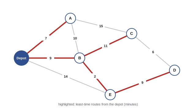
The result shows that the direct road from the depot to E (14 minutes) is not the fastest; going through B takes 11. The same algorithm, on networks of millions of nodes with refinements, powers navigation apps, emergency vehicle dispatch, and the routing of power flows and data packets. Engineers also use related graph algorithms: minimum spanning trees to connect sites with the least total pipe or cable length, maximum flow to find network capacity, and critical path analysis, which is a longest-path calculation on a schedule network.

Choosing algorithms in practice

For most engineering work, the practical lessons are:

• Use library functions (sorted, bisect, dictionaries and sets, NumPy, SciPy, networkx for graphs); they implement good algorithms carefully and are well tested.
• Think about how your program's work grows with data size before running it on a large dataset. Watch for nested loops over the same large collection and for repeated membership tests on lists.
• Vectorize numerical work with NumPy (Lesson 7).
• Measure before optimizing: Python's cProfile and the time module show where the time actually goes. Clear, correct code is worth more than fast, wrong code, and most programs are fast enough once the right algorithm and data structure are chosen.