Renewable resources and the changing grid

A year after his protection co-op term, Leo Tremblay is back at Larchmont Energy as an engineer-in-training in the distribution planning group. On his first morning his new supervisor, Marguerite LeBlanc, a planning engineer with fifteen years at the utility, drops a thick binder on his desk. It is an interconnection application from Birch Hill Energy: a 10 MW solar plant paired with a 5 MW, 20 MWh battery, proposed for farmland about 11 km (6.8 mi) from the Lincoln Road substation. Marguerite's instruction is short: \"By the end of the term I want you to be able to tell me whether we can connect it, what it will cost, and what we have to change. Start by understanding why this application is different from the ones we got twenty years ago.\"

This course follows Leo through that study. It is an electrical course: earlier courses treated wind, solar and storage as energy resources with costs and capacity factors, and the power electronics course taught how inverters and converters work inside. Here the question is what happens at the point where these resources meet the grid: how their electrical behavior differs from a synchronous generator, what the standards require of them, how a utility studies their effect on voltage, protection, power quality and frequency, and how they can be organized into microgrids and aggregations.

From central stations to distributed and inverter-based resources

For most of the twentieth century, electricity flowed one way. Large synchronous generators at hydro, coal, gas and nuclear stations fed a high-voltage transmission network, substations stepped the voltage down, and radial distribution feeders carried power outward to customers. Protection, voltage regulation and operating practice were all built on that pattern. A distribution feeder was a passive load, and its voltage fell steadily from the substation to the end of the line.

Two changes have overturned that picture. The first is the growth of distributed energy resources (DER): generation and storage connected to the distribution system, from rooftop solar of a few kilowatts to plants of 10 to 20 MW on dedicated feeders. The second is that almost all new wind, solar and battery capacity is inverter-based: it connects to the grid through power electronic converters rather than through the rotating magnetic field of a synchronous machine. These inverter-based resources (IBR) appear at every voltage level, from a 240 V house service to wind and solar plants connected at 230 kV.

The two changes are related but not the same. A 300 MW solar plant on the transmission system is an IBR but not a DER; a 2 MW diesel generator at a hospital is a DER but not an IBR. Many of the integration problems in this course come from one property or the other. Distribution-connected resources create reverse power flow and voltage rise on feeders that were never designed for them. Inverter-based resources behave differently from synchronous machines during faults and frequency disturbances, because their response is set by control software rather than by physics.

How inverter-based resources differ

A synchronous generator has a large spinning mass whose stored kinetic energy is released automatically when frequency falls. Its internal voltage stays nearly constant for the first few cycles after a fault, so it can supply five to ten times its rated current into a short circuit. It produces almost no harmonics, and its behavior during disturbances is fixed by its physical design, so it is the same in every plant of that type.

An inverter-based resource has none of these properties by default. Its power semiconductors are rated close to the plant's normal current, so fault current is typically limited to roughly 1.1 to 1.5 times rated, as lesson 9 discusses. It has no rotating mass coupled to the grid, so it does not slow the initial rate of change of frequency unless its controls are programmed to emulate inertia. It switches at kilohertz frequencies and must be filtered to keep harmonics low. And its response to every disturbance depends on firmware settings that differ between manufacturers, models and even firmware versions. That last point explains why grid codes and interconnection standards have become so detailed: they specify the behavior that physics no longer guarantees.

Inverters also bring advantages. They can change real and reactive power in milliseconds, far faster than any governor or exciter. They can supply reactive power at night if designed to do so. A battery inverter can switch from charging to discharging within a cycle or two. Much of this course is about turning those capabilities into services the grid needs, rather than treating inverter-based resources only as a problem to be contained.

The changing shape of load

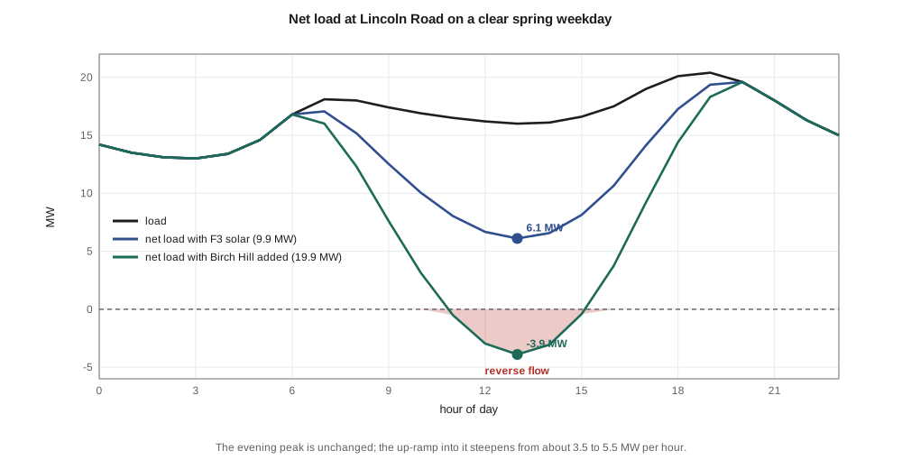
Leo's first task is to see what Birch Hill would do to the daily pattern at Lincoln Road. The substation already serves feeder F3, which carries a 9.9 MW solar plant that Leo met during his protection term. He takes a typical spring weekday load profile from the substation's SCADA history and a clear-sky solar profile, and computes the net load: the load that the transmission system must supply once local solar output is subtracted.

import math
# A spring weekday at Lincoln Road substation: hourly load and solar output (MW)
load = [14.2, 13.5, 13.1, 13.0, 13.4, 14.6, 16.8, 18.1, 18.0, 17.4, 16.9, 16.5,
        16.2, 16.0, 16.1, 16.6, 17.5, 19.0, 20.1, 20.4, 19.6, 18.0, 16.3, 15.0]
def solar(h, mw):                      # clear-day shape, sunrise 6 h, sunset 20 h
    if h <= 6 or h >= 20: return 0.0
    return mw*math.sin(math.pi*(h - 6)/14)**1.5
for case, pv in (('today: F3 solar only', 9.9), ('with Birch Hill (+10 MW)', 19.9)):
    net = [load[h] - solar(h, pv) for h in range(24)]
    hmin = min(range(24), key=lambda h: net[h])
    ramp = max(net[h + 1] - net[h] for h in range(23))
    print(f"{case:26s} min net load {net[hmin]:5.1f} MW at {hmin:02d}:00, "
          f"evening peak {max(net):4.1f} MW, steepest up-ramp {ramp:4.1f} MW/h")
# Light-load day (holiday, 7 MW midday load): does T1 (25 MVA) see reverse flow?
for pv in (9.9, 19.9):
    rev = pv*0.95 - 7.0                # 5 % losses and clipping on a clear noon
    print(f"PV {pv:4.1f} MW on a 7 MW holiday: flow at T1 = {-rev:+5.1f} MW "
          f"({'reverse' if rev > 0 else 'forward'}), {abs(rev)/25*100:3.0f} % of the transformer rating")

today: F3 solar only       min net load   6.1 MW at 13:00, evening peak 19.6 MW, steepest up-ramp  3.5 MW/h
with Birch Hill (+10 MW)   min net load  -3.9 MW at 13:00, evening peak 19.6 MW, steepest up-ramp  5.5 MW/h
PV  9.9 MW on a 7 MW holiday: flow at T1 =  -2.4 MW (reverse),  10 % of the transformer rating
PV 19.9 MW on a 7 MW holiday: flow at T1 = -11.9 MW (reverse),  48 % of the transformer rating

The results show the effect that planners in many regions now see every day. With the existing F3 plant, the substation's net load still dips to about 6 MW at midday. Adding Birch Hill's 10 MW pushes the midday minimum to about −4 MW: on a clear spring weekday, Lincoln Road would export power back into the 138 kV system. The evening peak is unchanged, because the sun has set by then, but the ramp from the midday trough to the evening peak becomes steeper, about 5.5 MW in one hour instead of 3.5 MW.

On a light-load holiday the reverse flow through the substation transformer would reach about 12 MW, nearly half of T1's 25 MVA rating. That is within the transformer's thermal capability, but it raises questions the utility must answer: whether the on-load tap changer and its controls work correctly with reverse flow, whether the 138 kV protection was set assuming power always flows into the station, and whether the transmission operator must be told. Each of those questions returns later in the course.

Who is involved in connecting a resource

An interconnection brings together several parties with different interests. The developer, or interconnection customer, wants to connect quickly and cheaply and to export as much energy as possible. The distribution utility must keep voltage, protection and power quality within limits for every other customer on the system. If the resource is large enough to affect the transmission system, the transmission owner and the system operator become involved. Regulators set the rules for applications, study timelines and how costs are shared.

In Wisconsin, distribution interconnections of 15 MW or less are governed by the Public Service Commission's rule PSC 119, revised in 2024. It sorts facilities into four categories by export capacity, from 20 kW or less up to 15 MW, each with its own application and study process, and it adopts IEEE 1547-2018 and the UL 1741 certification standard by reference. Larger resources, and those connecting to the transmission system, go through the Midcontinent Independent System Operator (MISO) queue under rules approved by the Federal Energy Regulatory Commission (FERC). Reliability standards for the bulk system are developed by the North American Electric Reliability Corporation (NERC).

Birch Hill sits near the boundary between these worlds. At 10 MW of solar and 5 MW of storage it is a distribution-connected resource, but at times it will push power up through Lincoln Road into the 138 kV system, so the transmission side cannot be ignored. Lessons 6 and 7 walk through the standards and the study process in detail.

Capacity, energy and the capacity factor

Two numbers describe a renewable plant, and confusing them is one of the most common mistakes in planning discussions. Capacity is the maximum power the plant can deliver, in megawatts. Energy is what it delivers over time, in megawatt-hours. The ratio of actual annual energy to what the plant would produce at full capacity all year is the capacity factor. A solar plant in New Brunswick or Wisconsin typically has a capacity factor in the mid-teens percent, a wind plant perhaps 30 to 40 %, and a hydro plant 40 to 60 %, depending on the site and design.

For grid integration, capacity often matters more than energy. Voltage rise, reverse flow and protection impacts depend on what the plant can inject at its maximum, usually around solar noon on a cool, clear day, regardless of how many hours a year it runs at that level. Planners therefore study the worst hour: maximum generation coinciding with minimum load. A plant with a modest capacity factor can still cause severe problems for a few hours a year.

What the grid needs from new resources

As inverter-based resources replace synchronous generators, the grid still needs the services that synchronous machines once supplied without anyone asking. These are often called essential reliability services. They include voltage support and reactive power; frequency response, both the fast initial response that limits how far frequency falls and the slower response that restores it; enough fault current for protection to work; and the ability to stay connected through disturbances rather than tripping and making them worse.

Modern standards require inverter-based resources to provide many of these services. They must ride through voltage and frequency disturbances, regulate voltage with reactive power, reduce output when frequency rises, and in some cases increase output when it falls. A newer class of grid-forming inverters, introduced in lesson 3, goes further by establishing voltage and frequency themselves instead of following the grid, which allows them to support weak grids and to run islanded microgrids.

Leo's study will touch all of these. The Birch Hill application includes a battery, which gives the plant flexibility a solar plant alone does not have: it can absorb midday power to reduce reverse flow, discharge into the evening ramp, and respond to frequency events. Whether the utility can use that flexibility depends on the interconnection agreement, the market rules and the controls, topics that return in lesson 12.