
ELE-390 · Lesson 8 of 12 · 23 min
Root-locus design with lead, lag and PID compensation
Lesson 7 ended with a diagnosis: proportional control cannot make the PT-1 pan servo settle fast enough, because the dominant root-locus branches are pinned near Re s = −10.6. It also gave the prescription: the desired pole location −20 + j26.6 misses the locus by 35.1°, so a compensator must add that much phase there. This lesson designs three compensators by root locus. A lead compensator reshapes the locus to meet the transient specification. A lag compensator, added to it, raises the velocity constant to meet the ramp specification without spoiling the transient. A PID controller, which turns out to be a close relative of lead-lag, adds integral action for the wind. The results are compared by simulation, including the motor voltage each one demands.
Compensators as poles and zeros
A first-order compensator has the form C(s) = K(s − z)/(s − p), one zero and one pole on the negative real axis. If the zero is closer to the origin than the pole, |z| < |p|, the compensator's phase is positive at every frequency: it is a lead compensator, because its output leads a sinusoidal input. If the pole is closer, |p| < |z|, it is a lag compensator. On the root locus, a zero pulls branches toward itself and a pole pushes them away. A lead compensator, with its zero closer to the origin, therefore pulls the dominant branches to the left, toward faster responses. A lag compensator, with its pole and zero both very close to the origin, barely changes the locus where the dominant poles are, but multiplies the DC gain by the ratio z/p.
The lead compensator is the practical form of derivative action. An ideal derivative, K_ds, adds 90° of phase and gain that rises without limit at high frequency, amplifying sensor noise. The lead's pole caps that gain at b/a times its low-frequency value. The lag compensator is the practical form of integral action: an ideal integrator has infinite DC gain, while a lag has a finite one, c/d, and so leaves the loop's type unchanged.
Designing the lead
There are several ways to place a lead compensator to supply a given phase. One of the simplest, when the plant has a well-known stable pole near the desired region, is to put the compensator's zero on top of that pole and cancel it. Amara puts the zero at −21.2, canceling the motor's mechanical pole. The loop gain then becomes, apart from the far electrical pole, 8.33K/(s(s + b)): the same form as before, but with the pole that was at −21 moved to −b. The breakaway point of that locus is at −b/2, so putting the dominant poles' real part at −20 requires b = 40.
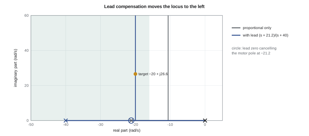
The angle condition confirms the choice. At s₀ = −20 + j26.6 the zero at −21.2 contributes +87.4° and the pole at −40 contributes −53.1°, a net 34.3°, within a degree of the 35.1° that lesson 7 asked for; the remaining fraction is the electrical pole's 0.8°. The magnitude condition gives the gain: with the electrical pole included, K = 130 V/rad puts a closed-loop pole exactly at s₀, and the simple model's value of 133 V/rad is close enough. The lead compensator is C(s) = 133(s + 21.2)/(s + 40).
Two consequences are worth noticing. First, the closed-loop transfer function is the same as the cascade of lesson 3: poles at −20 ± j26.6 and no closed-loop zero, because the compensator's zero canceled a plant pole rather than appearing in the closed loop. Second, the lead's high-frequency gain is K, so at the instant of a 10° step the motor voltage jumps to 133 × 0.1745 = 23.2 V, just inside the driver's ±24 V. A larger step would saturate the driver, a limit that lesson 12's trajectory planner removes.
Adding a lag
The lead design's velocity constant is K_v = 133 × (21.2/40) × 0.397 = 28.0 s⁻¹, far short of the 100 s⁻¹ the ramp specification needs. A lag compensator multiplies K_v by its DC gain c/d without moving the dominant poles much, provided its pole and zero are close together and close to the origin compared with the dominant poles. A ratio c/d = 4 raises K_v to about 112 s⁻¹.
The placement is a trade-off. The lag adds a slow closed-loop pole near its zero, and that pole's mode appears as a slow tail in the step response. Its size is roughly proportional to how far the closed-loop pole is from the lag zero, which shrinks as the lag pair moves toward the origin, but its duration grows. A lag zero at −2, one tenth of the dominant real part, a common textbook rule, leaves a tail large enough to push the 2 % settling time past 0.5 s. Amara moves the pair to a zero at −0.5 and a pole at −0.125, keeps the ratio at 4, and trims the overall gain to 120 V/rad to bring the overshoot back under 10 %.
PID by root locus
The lag compensator still leaves the loop type 1. It reduces the wind error by a factor of four, but does not remove it. Moving the lag's pole all the way to the origin turns it into an integrator, and the compensator becomes K(s + 21.2)(s + c)/(s(s + 40)). Expanding that product shows it is a PID controller whose derivative term has a first-order filter with a time constant of 25 ms: a proportional, an integral and a filtered derivative term, combined. The root-locus view of PID is exactly this pair of zeros, one placed for transient response, one for steady-state error, plus an integrator pole at the origin and a filter pole far to the left.
The integrator pole at the origin, with its zero at −c, adds a slow closed-loop pole between them, just as the lag did, but this time the pole cannot be pushed arbitrarily close to its zero without weakening the integral action. Amara tries c = −1, −2 and −3 in simulation and picks c = 2 with K = 125 as the best compromise, then compares all three designs.
import math, cmath
R, L, Kt, J, b, N = 2.0, 1e-3, 0.05, 6e-5, 1e-5, 50
deg = math.pi / 180
# controllers as lists of first-order sections (zero, pole): C(s) = K * prod (s - z)/(s - p)
def make(K, sections):
    def init(): return [0.0] * len(sections)
    def step(x, e, dt):
        v = e
        for k, (z, p) in enumerate(sections):
            # (s - z)/(s - p) = 1 + (p - z)/(s - p); state x' = p x + v
            out = v + (p - z) * x[k]
            x[k] += dt * (p * x[k] + v)
            v = out
        return K * v
    return init, step
def sim(ctrl, r=0.0, ramp=0.0, Td=0.0, t_end=2.0, dt=5e-5, vmax=None):
    init, step = ctrl; x = init(); i = wm = th = 0.0; t = 0.0; ys = []; umax = 0.0
    while t < t_end:
        e = r + ramp * t - th
        u = step(x, e, dt)
        if vmax: u = max(-vmax, min(vmax, u))
        umax = max(umax, abs(u))
        i += dt * (u - R * i - Kt * wm) / L
        wm += dt * (Kt * i - b * wm - Td / N) / J
        th += dt * wm / N; t += dt; ys.append((t, th))
    return ys, umax
def metrics(ys, r):
    peak = max(y for _, y in ys)
    ts = max((t for t, y in ys if abs(y - r) > 0.02 * r), default=0.0)
    return 100 * (peak / r - 1), ts
designs = {
    "lead":          (133.0, [(-21.2, -40.0)]),
    "lead-lag":      (120.0, [(-21.2, -40.0), (-0.5, -0.125)]),
    "lead-PI (PID)": (125.0, [(-21.2, -40.0), (-2.0, 0.0)]),
}
for name, (K, sec) in designs.items():
    ctrl = make(K, sec)
    ys, umax = sim(ctrl, r=10 * deg, t_end=4.0)
    Mp, ts = metrics(ys, 10 * deg)
    ramp, _ = sim(make(K, sec), ramp=20 * deg, t_end=25.0, dt=1e-4)
    wind, _ = sim(make(K, sec), Td=1.5, t_end=25.0, dt=1e-4)
    C0 = K * math.prod(z / p for z, p in sec) if all(p != 0 for _, p in sec) else float('inf')
    Kv = C0 * 0.3968
    kv = f"{Kv:6.1f}" if Kv < 1e9 else "   inf"
    print(f"{name:14s} overshoot {Mp:5.1f} %, settling {ts*1000:4.0f} ms, peak voltage {umax:5.1f} V, Kv {kv}, "
          f"ramp error {abs(20*deg*ramp[-1][0] - ramp[-1][1])/deg:5.3f} deg, wind error {abs(wind[-1][1])/deg:5.3f} deg")
# angle and gain check of the lead design at the target point, including the electrical pole
s0 = complex(-20, 26.6)
G = lambda s: 16667 / (s * (s + 21.2) * (s + 1979))
Cl = lambda s: (s + 21.2) / (s + 40)
print(f"angle of C*G at s0: {math.degrees(cmath.phase(Cl(s0) * G(s0))):.1f} deg; gain for a pole there {1/abs(Cl(s0)*G(s0)):.0f}")lead overshoot 10.0 %, settling 177 ms, peak voltage 23.2 V, Kv 28.0, ramp error 0.715 deg, wind error 0.975 deg lead-lag overshoot 9.9 %, settling 207 ms, peak voltage 20.9 V, Kv 100.9, ramp error 0.198 deg, wind error 0.270 deg lead-PI (PID) overshoot 17.3 %, settling 703 ms, peak voltage 21.8 V, Kv inf, ramp error 0.000 deg, wind error 0.000 deg angle of C*G at s0: 179.2 deg; gain for a pole there 130
Comparing the designs
| Design | Overshoot | 2 % settling | Peak voltage | K_v (s⁻¹) | Ramp error at 20°/s | Wind error |
|---|---|---|---|---|---|---|
| Lead, K = 133 | 10.0 % | 177 ms | 23.2 V | 28.0 | 0.72° | 0.98° |
| Lead-lag, K = 120 | 9.9 % | 207 ms | 20.9 V | 101 | 0.20° | 0.27° |
| Lead-PI (PID), K = 125 | 17.3 % | 703 ms | 21.8 V | ∞ | 0 | 0 |
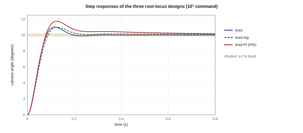
The lead-lag compensator meets every specification of lesson 1 except one: overshoot 9.9 %, settling 207 ms, K_v of 101 s⁻¹ and a ramp error of 0.198°, all within the limits, with a peak voltage of 20.9 V. The wind error is 0.27°, small but not zero. The lead-PI design removes both steady errors entirely, but its overshoot is 17.3 % and it takes 0.7 s to settle, because the integrator's closed-loop pole and zero sit near −2 and leave a tail that the eye can see. The comparison illustrates a general truth about one-degree-of-freedom controllers: the same compensator shapes the response to both commands and disturbances, and the integral action that is so effective against the wind slows the step response.
The lead design is also worth comparing with lesson 3's cascade, which has identical closed-loop poles. The two follow commands identically, but the lead's wind error is 0.98°, almost twice the cascade's 0.52°. The difference is the DC gain each presents to the disturbance: the cascade applies its full K_p = 133 V/rad to a steady error, while the lead's DC gain is 133 × 21.2/40 = 70.5 V/rad. Two controllers with the same closed-loop poles can differ in everything else, which is why a design is never finished at the pole locations.
Worked problem
A lead compensator without cancellation
For the tilt axis, with plant G(s) = 600/(s(s + 15)(s + 120)), the desired dominant poles are at −16 ± j15.4 (lesson 4). Place the lead zero at −16, directly below the desired point, and find the pole location that supplies the required phase, and the gain.
Show solution
- Angle of G at s₀ = −16 + j15.4: −(136.1° + 93.7° + 8.4°) = −238.2°, so the lead must add 58.2°.
- The zero at −16 contributes 90°, so the pole must contribute 90° − 58.2° = 31.8°: its distance to the left of −16 is 15.4/tan 31.8° = 24.9, so the pole is at −40.9.
- \[K = \frac{|s_0|\,|s_0 + 15|\,|s_0 + 120|\,|s_0 + 40.9|}{600\,|s_0 + 16|} = \frac{22.2 \times 15.4 \times 105.1 \times 29.3}{600 \times 15.4} \approx 114\]
- Check the third closed-loop pole and simulate before accepting the design; the zero at −16 also appears in the closed loop and adds overshoot.
Answer: C(s) ≈ 114(s + 16)/(s + 40.9) V/rad. Placing the zero directly below the target is a quick alternative when there is no plant pole worth canceling.
When cancellation is safe
The lead design canceled the motor pole at −21.2. That is safe because the pole is stable and well known, and because exact cancellation is not required: if the real motor's pole is at −19 or −24, the compensator's zero sits close to it, the closed loop gains a pole and zero close together, and lesson 4 showed that such a pair has little effect. Leo measured the mechanical time constant of five prototype motors and found a spread of ±8 %, which moves the dominant poles by less than a degree in angle. Daniel adds a check to the test procedure: measure the step response of every production unit at power-up, and flag any whose overshoot exceeds 15 %. Cancellation of a lightly damped pole, such as a structural resonance, or of any right-half-plane pole would not be safe, for the reasons lesson 3 gave.
Implementing the compensators
In the PT-1 the compensators are implemented in the microcontroller as difference equations, which lesson 11 derives. A lead compensator can also be built as an analog circuit: an op-amp with an RC network in its input path, with the zero at 1/(R₁C₁) and the pole at (R₁ + R₂)/(R₁R₂C₁), as in the lead networks used in analog servo amplifiers for decades. Either way, the design in the s-plane comes first, and the implementation must preserve its poles and zeros to within the tolerances the design can absorb.
Common mistakes
MistakePlacing the lag zero close to the dominant poles.
InsteadKeep the lag pair near the origin, roughly one tenth of the dominant real part or closer, and check the settling tail.
MistakeAssuming two designs with the same closed-loop poles reject disturbances equally.
InsteadDisturbance rejection depends on the controller's gain at the disturbance frequency, not only on the poles.
MistakeForgetting to check actuator effort.
InsteadA lead's high-frequency gain sets the voltage at the instant of a step; check against the driver limit.
MistakeCanceling poles that are poorly known or lightly damped.
InsteadCancel only stable, well-characterized poles; otherwise place the zero nearby and verify robustness.
Summary and key terms
- A lead compensator (zero nearer the origin than its pole) adds phase and pulls the root locus left; a lag compensator multiplies the DC gain with little change to the dominant poles.
- Canceling the motor pole at −21.2 with a lead zero and placing its pole at −40 moves the vertical part of the locus to −20; K = 133 V/rad meets the transient specification.
- A lag with zero −0.5, pole −0.125 and K = 120 V/rad raises K_v to 101 s⁻¹, meeting the ramp specification with 9.9 % overshoot and 207 ms settling.
- Moving the lag pole to the origin gives a PID controller with a filtered derivative; it removes the ramp and wind errors but raises overshoot to 17 % and slows settling.
- Designs with the same closed-loop poles can differ in disturbance rejection and actuator effort; simulate both.
- Pole-zero cancellation is safe only for stable, well-known poles.
- Compensator
- A dynamic element added to a loop to change its root locus or frequency response.
- Lead compensator
- K(s + a)/(s + b) with a < b, adding phase to speed the response.
- Lag compensator
- (s + c)/(s + d) with d < c, raising low-frequency gain with little phase change near crossover.
- Lead-lag compensator
- A lead and a lag in series, shaping both transient and steady-state behavior.
- PID controller
- A controller with proportional, integral and derivative terms; in practice the derivative is filtered.
- Derivative filter
- A pole that limits the derivative term's gain at high frequency.
- Pole-zero cancellation
- Placing a compensator zero on a plant pole, or the reverse, so that they cancel in the loop gain.
- Actuator effort
- The control signal a design demands, such as motor voltage.
Practice problems
Work each problem on paper first, then reveal the answer to check.
A lead C(s) = 50(s + 10)/(s + 50) is used with a 10° step. What voltage appears at the first instant?
Show answer
The high-frequency gain is 50, so 50 × 0.1745 = 8.7 V.
What is the DC gain of the lag (s + 0.5)/(s + 0.125)?
Show answer
0.5/0.125 = 4.
Find the velocity constant of 120(s + 21.2)(s + 0.5)/((s + 40)(s + 0.125)) × 0.397/s × 21/(s + 21), approximately.
Show answer
120 × 0.53 × 4 × 0.397 ≈ 101 s⁻¹.
Write K(s + 21.2)(s + 2)/(s(s + 40)) with K = 125 in PID form at low frequency.
Show answer
K_I = 125 × 21.2 × 2/40 = 132.5 V/(rad·s); K_P and K_D follow from partial fractions.
Why does the lead-PI design overshoot more than the lead-lag?
Show answer
The integrator's zero at −2 is closer to the dominant poles than the lag's, and its slow closed-loop pole leaves a larger tail.
Which pole of the pan plant is safe to cancel, and which kinds of poles are not?
Show answer
The stable, well-measured motor pole at −21.2; lightly damped or unstable poles are not.
Lesson quiz · 5 questions
Score 60% or more to complete this lesson.
Create a free account to save your progress, take quizzes and earn a certificate.