Frequency-domain design and stability margins

Lesson 9 showed how to read stability and performance from the loop gain's frequency response. This lesson designs with it. Frequency-domain design, often called loop shaping, chooses a compensator so that the loop gain has the right shape: high at low frequency, falling through 0 dB on a gentle slope with enough phase margin, and low at high frequency. The lead and lag compensators of lesson 8 reappear, now placed by their effect on gain and phase rather than on the root locus. The lesson also does something the root locus does poorly: it accounts for the effects the model left out, the controller's sampling delay, a resonance in the camera bracket and the spread of parameters between units, and asks whether the PT-1 design still has the margins Daniel's review requires.

Specifications in the frequency domain

The specifications of lesson 1 translate into frequency-domain targets. The velocity constant K_v is the low-frequency asymptote of the loop gain: for a type 1 loop, |L(jω)| ≈ K_v/ω at low frequency, so K_v = 100 s⁻¹ means the −20 dB/decade line passes through 0 dB at ω = 100 rad/s when extended. The overshoot and damping requirement becomes a phase margin, about 60° for ζ ≈ 0.6. The settling time becomes a crossover frequency, roughly ω_c ≈ 8/t_s to 10/t_s, so 0.25 s asks for something like 30 to 40 rad/s, and less if the phase margin is high. Robustness becomes the margins themselves, at least 50° and 10 dB for the PT-1, and a peak sensitivity |S|_max, which should not exceed about 1.5 to 2.

The peak sensitivity deserves its place in the list. It is the reciprocal of the shortest distance from the Nyquist plot to the point −1, so it captures gain and phase margin in one number: |S|_max ≤ 1.5 guarantees a gain margin of at least 9.5 dB and a phase margin of at least 39°. It is also the worst-case amplification of disturbances at any frequency. Modern practice often specifies it directly.

Lead design on the Bode plot

The lead compensator C(s) = K(s/z + 1)/(s/p + 1) adds positive phase between its zero and pole, with a maximum φ_max at the geometric mean ω_m = √(zp). Writing α = z/p < 1, the maximum phase satisfies sin φ_max = (1 − α)/(1 + α), and at ω_m the lead raises the gain by 1/√α. The classical Bode procedure is: set the gain K to meet the steady-state requirement; find the phase margin of K·G; add a lead supplying the missing phase plus a few degrees of allowance, since the lead's gain moves the crossover to a higher frequency where the plant has more lag; and place ω_m at the new crossover, where the uncompensated gain is −10 log(1/α) dB.

Amara follows the procedure for the PT-1 as a cross-check on lesson 8. She sets K = 100/0.397 = 252 V/rad for K_v = 100, finds the phase margin of the uncompensated loop and designs the lead.

import math, cmath
def G(s, Jscale=1.0, kscale=1.0):
    # pan plant volts -> radians; inertia scaling moves the mechanical pole (back-emf damping fixed)
    p_mech = 21.2 / Jscale
    return kscale * 16667 / Jscale / (s * (s + p_mech) * (s + 1979))
def margins(L, wlo=0.05, whi=3000.0, n=6000):
    """Crossover, phase margin, worst gain margin over all phase crossings, and peak sensitivity."""
    ws = [wlo * (whi / wlo) ** (k / n) for k in range(n + 1)]
    ph, prev, data = 0.0, None, []
    for w in ws:
        v = L(1j * w); p = cmath.phase(v)
        if prev is not None:
            d = p - prev
            while d > math.pi: d -= 2 * math.pi
            while d < -math.pi: d += 2 * math.pi
            ph += d
        else: ph = p
        prev = p; data.append((w, abs(v), math.degrees(ph)))
    k = next(i for i, (w, m, p) in enumerate(data) if m < 1)
    lo, hi = data[k - 1][0], data[k][0]
    for _ in range(60):                                   # refine the gain crossover
        mid = math.sqrt(lo * hi)
        lo, hi = (mid, hi) if abs(L(1j * mid)) > 1 else (lo, mid)
    wc = lo; pm = 180 + data[k][2] + math.degrees(cmath.phase(L(1j * wc)) - cmath.phase(L(1j * data[k][0])))
    gm = min((-20 * math.log10(m2) for (w1, m1, p1), (w2, m2, p2) in zip(data, data[1:])
              if math.floor((p1 + 180) / 360) != math.floor((p2 + 180) / 360)), default=float('inf'))
    ms = max(1 / abs(1 + L(1j * w)) for w, _, _ in data)
    return wc, pm, gm, ms
# 1. Bode design: gain for Kv = 100, then a lead for 55 deg of phase margin
K = 100 / 0.3968
wc0, pm0, _, _ = margins(lambda s: K * G(s))
phi = math.radians(55 - pm0 + 8)                     # 8 deg allowance for the crossover shift
alpha = (1 - math.sin(phi)) / (1 + math.sin(phi))
# put the lead's maximum phase at the new crossover, where the uncompensated gain is -10 log(1/alpha)
target = math.sqrt(alpha)
lo, hi = 1.0, 1000.0
for _ in range(80):
    mid = math.sqrt(lo * hi)
    lo, hi = (mid, hi) if abs(K * G(1j * mid)) > target else (lo, mid)
wm = lo; z, p = wm * math.sqrt(alpha), wm / math.sqrt(alpha)
Cb = lambda s: K * (s / z + 1) / (s / p + 1)
wc, pm, gm, ms = margins(lambda s: Cb(s) * G(s))
print(f"uncompensated K = {K:.0f}: crossover {wc0:.1f} rad/s, PM {pm0:.1f} deg")
print(f"lead alpha = {alpha:.3f}: zero {z:.1f}, pole {p:.1f} rad/s; crossover {wc:.1f}, PM {pm:.1f} deg, peak |S| {ms:.2f}")
print(f"high-frequency gain {K*p/z:.0f} V/rad -> {K*p/z*math.radians(10):.0f} V at the instant of a 10 deg step")
# 2. the lesson 8 lead-lag with the things the model left out
Cll = lambda s: 120.0 * (s + 21.2) * (s + 0.5) / ((s + 40) * (s + 0.125))
Td = 0.5e-3 + 0.3e-3                                  # zero-order hold plus computation
wr, zr = 260.0, 0.02                                  # camera bracket torsional mode
res = lambda s: wr**2 / (s * s + 2 * zr * wr * s + wr**2)
cases = [("model", lambda s: Cll(s) * G(s)),
         ("+ 0.8 ms delay", lambda s: Cll(s) * G(s) * cmath.exp(-Td * s)),
         ("+ delay + bracket mode", lambda s: Cll(s) * G(s) * cmath.exp(-Td * s) * res(s)),
         ("heated housing (+40 % J)", lambda s: Cll(s) * G(s, 1.4) * cmath.exp(-Td * s) * res(s)),
         ("weak motor (-20 % gain)", lambda s: Cll(s) * G(s, 1.0, 0.8) * cmath.exp(-Td * s) * res(s)),
         ("strong motor (+20 % gain)", lambda s: Cll(s) * G(s, 1.0, 1.2) * cmath.exp(-Td * s) * res(s))]
for name, L in cases:
    wc, pm, gm, ms = margins(L)
    print(f"{name:27s} crossover {wc:5.1f} rad/s, PM {pm:5.1f} deg, GM {gm:5.1f} dB, peak |S| {ms:.2f}")
# 3. how close does the bracket resonance come to the critical point?
L = lambda s: Cll(s) * G(s) * cmath.exp(-Td * s) * res(s)
v = L(1j * wr)
print(f"at the bracket mode, 260 rad/s: |L| = {20*math.log10(abs(v)):.1f} dB at {math.degrees(cmath.phase(v)) % 360 - 360:.0f} deg")

uncompensated K = 252: crossover 43.7 rad/s, PM 24.6 deg
lead alpha = 0.234: zero 31.2, pole 133.5 rad/s; crossover 64.6, PM 54.7 deg, peak |S| 1.39
high-frequency gain 1078 V/rad -> 188 V at the instant of a 10 deg step
model                       crossover  22.1 rad/s, PM  59.5 deg, GM  38.0 dB, peak |S| 1.35
+ 0.8 ms delay              crossover  22.1 rad/s, PM  58.4 deg, GM  29.7 dB, peak |S| 1.38
+ delay + bracket mode      crossover  22.2 rad/s, PM  58.1 deg, GM  24.2 dB, peak |S| 1.39
heated housing (+40 % J)    crossover  19.2 rad/s, PM  52.1 deg, GM  26.4 dB, peak |S| 1.44
weak motor (-20 % gain)     crossover  18.5 rad/s, PM  62.5 deg, GM  26.1 dB, peak |S| 1.32
strong motor (+20 % gain)   crossover  25.7 rad/s, PM  54.2 deg, GM  22.6 dB, peak |S| 1.45
at the bracket mode, 260 rad/s: |L| = -8.7 dB at -281 deg

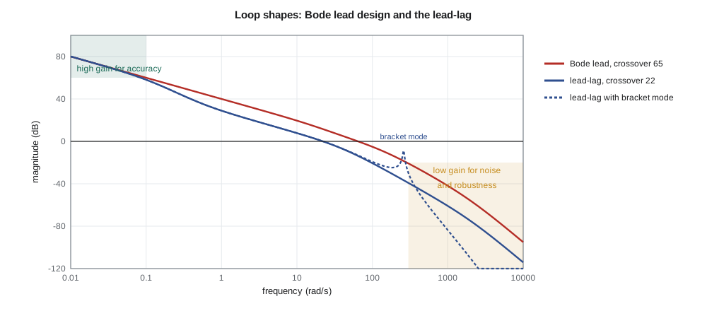
The uncompensated loop at K = 252 V/rad crosses over at 43.7 rad/s with only 24.6° of phase margin. A lead with α = 0.234, zero at 31.2 rad/s and pole at 133.5 rad/s brings the margin to 54.7° at a crossover of 64.6 rad/s, with a peak sensitivity of 1.39. On paper it is a better design than lesson 8's: three times the crossover, and the velocity constant met without a lag. But its high-frequency gain is K/α = 1078 V/rad, so a 10° step demands 188 V from a 24 V driver. The design is meaningless for steps of that size; it would spend most of each move saturated, behaving like a different and much slower system. For tiny corrections it would work, and it would amplify encoder quantization noise by the same factor of 1078 V/rad, putting audible chatter into the motor.

The comparison teaches the most important lesson of frequency-domain design: the crossover frequency is set by what the actuator and sensor can support, not only by the plant. Lesson 8's lead-lag crosses over at 22 rad/s with a high-frequency gain of 120 V/rad, uses at most 21 V for a 10° step, and meets the settling specification with a little to spare. Lesson 12 returns to the faster design and shows how a trajectory planner lets the servo be fast without demanding impossible voltages.

Lag design on the Bode plot

In the frequency domain a lag compensator (s/c + 1)/(s/d + 1), with d < c, raises the gain below d by c/d and leaves it nearly unchanged above c, at the cost of some phase lag between them. The procedure is to design the loop for its transient behavior first, then add the lag with its zero about a decade below the crossover frequency, so that its phase lag at crossover is only a few degrees, and with the ratio c/d set by how much low-frequency gain is needed. Lesson 8's lag, zero at 0.5 rad/s and pole at 0.125 rad/s, has its zero more than a decade below the 22 rad/s crossover and costs about 1° of phase there. The low-frequency gain rises by four, and the loop gain at 0.1 rad/s is 58 dB.

What the model left out

Three effects are missing from the transfer function that lessons 7 to 9 used. The first is delay. The controller samples the encoder and updates the motor voltage once per millisecond, and a zero-order hold delays a signal by half a sample on average, 0.5 ms. Computing the control law takes about 0.3 ms more. A total delay of 0.8 ms costs 0.8 × 10⁻³ × 22 rad = 1.0° of phase at the 22 rad/s crossover, which is trivial, but 9.2° at 200 rad/s, near the phase crossover, where it matters. The second is a structural resonance. Leo's swept-sine measurement on the prototype shows a sharp peak near 260 rad/s, about 41 Hz, which he traces to torsion of the camera bracket against the inertia of the housing; he models it as a second-order pair with ζ ≈ 0.02, a resonant peak of about 28 dB. The third is the spread of parameters: the heated housing adds 40 % to the inertia, and the motor's torque constant varies by up to ±20 % with temperature and between units.

The code applies each effect to the lead-lag design in turn. Delay cuts the gain margin from 38.0 dB to 29.7 dB and the phase margin by 1°. The bracket mode cuts the gain margin to 24.2 dB. The heated housing lowers the crossover to 19.2 rad/s and the phase margin to 52.1°; a strong motor raises the crossover to 25.7 rad/s and lowers the phase margin to 54.2° and the gain margin to 22.6 dB. In every case the margins stay above Daniel's 50° and 10 dB, and the peak sensitivity stays below 1.5. The design is robust to everything Leo has measured.

The bracket mode deserves a closer look. At 260 rad/s the loop gain, including the resonant peak, reaches −8.7 dB, within 9 dB of 0 dB. The loop is safe only because its phase there is about −281°, so the resonance swings the Nyquist plot in a small loop that passes on the far side of the origin from −1. A resonance whose stability depends on its phase is called phase-stabilized; one whose peak stays well below 0 dB whatever its phase is gain-stabilized. Phase stabilization is fragile, because a small change in delay or in the resonance frequency can rotate the loop toward −1. Daniel asks for a notch filter in the firmware, centered on the bracket mode, as a precaution for heavier cameras, and for the bracket to be stiffened in the next revision so that the mode moves above 500 rad/s.

Bandwidth, noise and the encoder

Every decibel of loop gain above crossover passes sensor noise to the actuator. The PT-1's encoder quantizes the angle to 0.0036°, or 63 µrad, and the controller's proportional path converts that to voltage: at 120 V/rad a single count is 7.5 mV, inaudible. The Bode lead design's 1078 V/rad would turn one count into 68 mV of square-wave chatter at the sampling rate, which is audible in the gearbox and wears it. Quantization noise is broadband, so the noise reaching the motor is set by the controller's high-frequency gain, the gain above crossover, which is one more reason to keep the crossover only as high as the specifications need.

The same reasoning sets the derivative filter in a PID controller and the pole of a lead compensator. The derivative term's gain must be capped at a frequency comfortably above crossover, typically 5 to 10 times, so that it adds phase where it is needed without amplifying noise where it is not. Lesson 8's lead pole at 40 rad/s, about twice the crossover, is on the conservative side, which costs a little phase margin and keeps the motor quiet.

Loop shaping as a design philosophy

The methods of lessons 8 and 10 are two views of the same design. The root locus is natural when the specifications are about pole locations and the plant model is trusted; the Bode plot is natural when the specifications are about margins, bandwidth and noise, and when the plant is known partly from measurement. Experienced designers move between them. A modern formalization of loop shaping, H-infinity control, chooses the controller to bound weighted versions of S and T at all frequencies, and leads to the same picture: high gain where accuracy is needed, low gain where the model is uncertain or the sensor is noisy, and a well-behaved crossover in between. The fundamental limits are the same too. Bode showed that for a stable loop the area under ln|S(jω)| is zero, so reducing sensitivity at some frequencies must increase it at others, a result sometimes called the waterbed effect.