Transfer functions and block diagrams

Lesson 2 produced differential equations for the PT-1 pan drive and the CC-1 cabinet. Differential equations are awkward to combine: connect a controller to a plant, add a sensor and a disturbance, and the equations multiply. Transfer functions make the combination algebraic. Each block in a diagram becomes a ratio of polynomials in s, connections become products and sums, and a feedback loop becomes a single division. This lesson reviews the transfer function from ELE-250, builds the algebra of block diagrams, and uses it to draw the pan servo with a velocity loop inside a position loop and to find how much the wind pushes the camera off target.

Transfer functions, poles and zeros

The transfer function of a linear time-invariant system is the Laplace transform of its output divided by the Laplace transform of its input, with all initial conditions zero. It is also the Laplace transform of the impulse response. For systems described by ordinary differential equations with constant coefficients it is a ratio of polynomials, and its numerator and denominator roots are the system's zeros and poles.

The poles determine the natural modes of the response: a real pole at −a contributes e^{−at}, and a complex pair at −σ ± jω_d contributes a decaying oscillation e^{−σt} sin(ω_d t + φ). A system is stable when every pole has a negative real part, as ELE-250 showed. The zeros do not create modes of their own, but they change how much of each mode appears. The degree n of the denominator is the order of the system; physical systems have n ≥ m, and most control plants have more poles than zeros, which is why their gain falls at high frequency.

Two numbers are read straight off a transfer function. The DC gain, G(0), is the steady output per unit of a constant input, provided the system is stable. The cabinet's G(s) = 0.1/(3000s + 1) has a DC gain of 0.1 K/W: a steady 100 W raises the temperature by 10 K. The PT-1's position plant G(s) = 8.33/(s(s + 21.0)) has no finite DC gain because of its pole at the origin: a constant voltage produces a constant speed, so the angle ramps without limit. That integrator is a defining feature of position servos.

Block diagram algebra

A block diagram shows signals as arrows and transfer functions as boxes. Three connections cover almost every case. Blocks in series multiply: the output of G₁ feeds G₂, so the combination is G₁G₂. Blocks in parallel, whose outputs are added at a summing junction, add: G₁ + G₂. A feedback connection, where the output of G is fed back through H and subtracted from the input, reduces to G/(1 + GH). The last rule follows from the same algebra as lesson 1: y = G e and e = r − Hy, so y = Gr/(1 + GH).

The product GH is the loop gain L. When H = 1 the loop has unity feedback, and the closed-loop transfer function is L/(1 + L), the complementary sensitivity T of lesson 1. When H is a sensor with its own dynamics, the closed loop is G/(1 + GH), and the steady output follows r/H rather than r: a sensor that reads 2 % high makes the output settle 2 % low.

Two more manipulations help simplify diagrams. A summing junction can be moved past a block if the signals entering it are adjusted: moving a junction from after G to before G divides the added signal by G. A pickoff point, where a signal branches, can be moved past a block in the same way, multiplying or dividing the branch. With these moves any diagram of interconnected loops can be reduced step by step to a single transfer function.

Several inputs: superposition

A real loop has more than one input. The pan servo has the commanded angle, the wind torque and the encoder's quantization noise. Because the system is linear, each input's effect can be found separately with the others set to zero, and the results added. The transfer function from reference to output is T; from an output disturbance to output it is S; from sensor noise to output it is −T. A disturbance entering somewhere in the middle of the plant, as the wind torque does, has its own transfer function, found by tracing the loop from where it enters.

Here G_d is the transfer function from the disturbance to the output with the loop open. All three closed-loop transfer functions share the denominator 1 + CG, so they share the same poles. That is an important fact: the stability and the transient character of a loop are the same whichever input excites it. The numerators differ, which is why a loop can follow commands well and still reject disturbances poorly, or the reverse.

The pan servo with a rate loop

Amara's first attempt at the pan controller, in lesson 1's terms, is pure proportional control: a voltage of K_p volts per radian of error. With K_p = 27 V/rad the closed-loop transfer function is 224.9/(s² + 21s + 224.9), whose poles are at −10.5 ± j10.7. As lesson 4 will show, that is a damping ratio of 0.70, a well damped response, but a slow one, taking about 0.38 s to settle. Raising K_p speeds the response but reduces the damping, because the only damping in the loop is the motor's own.

A common remedy is a second, inner loop that feeds back the camera's speed. The encoder already gives position; differentiating it in the controller, with filtering, gives a speed estimate. The inner loop applies a voltage proportional to speed with gain K_d, which acts like extra viscous friction that the designer can choose. The outer loop then closes on position with gain K_p around the damped inner loop. This cascade structure appears throughout motion control: current loop inside velocity loop inside position loop, each faster than the one around it.

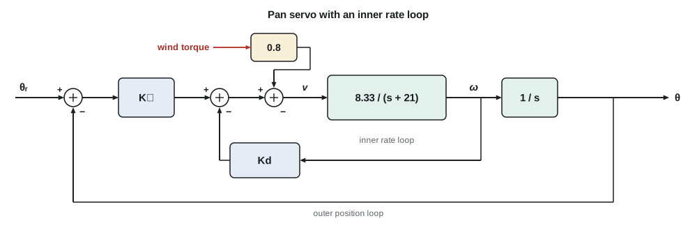
Reducing the diagram from the inside out is mechanical. The inner loop is G_ω = 8.33/(s + 21) with feedback K_d, giving 8.33/(s + 21 + 8.33K_d). The integrator 1/s follows. The outer loop then closes around K_p times that product, giving a second-order closed loop whose damping term the designer now controls through K_d.

To place the poles at −20 ± j26.6, Amara needs 8.33K_p = 20² + 26.6² ≈ 1108 and 21 + 8.33K_d = 40. That gives K_p = 133 V/rad and K_d = 2.28 V per rad/s. Lesson 4 shows that those poles give 10 % overshoot and a settling time of 0.2 s, which meets the transient specification of lesson 1. Lesson 8 shows that the same result can be obtained from a single controller placed in the forward path, and explains when the two arrangements differ.

The wind torque

The wind acts on the camera housing, not on the voltage, so its path into the loop must be traced through the plant. Lesson 2's motor equation has the load torque T_d/N entering the mechanical side. Neglecting the electrical pole, the current is (v − K_eω)/R, so a torque T_d at the camera has the same effect as a voltage of T_d R/(K_t N) subtracted at the motor terminals. For the PT-1 that factor is 2.0/(0.05 × 50) = 0.8 V per N·m. A 20 m/s gust on the housing, with its center of pressure offset from the pan axis, produces something like 1.5 N·m, equivalent to 1.2 V.

import cmath
# polynomials as coefficient lists, highest power first
def pmul(a, b):
    out = [0.0] * (len(a) + len(b) - 1)
    for i, x in enumerate(a):
        for j, y in enumerate(b): out[i + j] += x * y
    return out
def padd(a, b):
    n = max(len(a), len(b)); a = [0.0] * (n - len(a)) + a; b = [0.0] * (n - len(b)) + b
    return [x + y for x, y in zip(a, b)]
def peval(p, s):
    v = 0
    for c in p: v = v * s + c
    return v
def feedback(num, den, hnum=[1.0], hden=[1.0]):
    """Closed loop G/(1 + GH) for G = num/den and H = hnum/hden."""
    return pmul(num, hden), padd(pmul(den, hden), pmul(num, hnum))
def roots2(p):
    a, b, c = p
    d = cmath.sqrt(b * b - 4 * a * c)
    return (-b + d) / (2 * a), (-b - d) / (2 * a)
G = ([8.33], [1.0, 21.0, 0.0])                  # volts to camera radians
show = lambda p: ' '.join(f"{c:+.4g}" for c in p)
# 1. proportional position control, Kp = 27 V/rad
num, den = feedback([27 * 8.33], G[1])
print("P control:   T(s) =", show(num), "/", show(den), " poles", [f"{r:.2f}" for r in roots2(den)])
# 2. inner rate loop (Kd V per rad/s) inside an outer position loop (Kp V/rad)
Kp, Kd = 133.0, 2.28
inner = feedback(G[0], G[1], [Kd, 0.0])          # rate feedback Kd*s
outer = feedback(pmul([Kp], inner[0]), inner[1])
den = outer[1][-3:] if abs(outer[1][0]) < 1e-12 else outer[1]
print("rate + position: den", show(outer[1]), " poles", [f"{r:.2f}" for r in roots2(outer[1][-3:])])
# 3. disturbance: wind torque Td at the camera enters as 0.8*Td volts at the motor
R, Kt, N = 2.0, 0.05, 50
kd = R / (Kt * N)
print(f"torque-to-voltage factor R/(Kt N) = {kd:.2f} V per N*m")
for name, Kpos, Krate in (("P only", 27.0, 0.0), ("rate + position", Kp, Kd)):
    # theta/Td = -kd*G / (1 + G*(Kpos + Krate*s)); at s = 0 the G's integrator cancels
    err = kd * 1.5 / Kpos
    print(f"{name:16s}: 1.5 N*m gust -> steady error {err*1000:.1f} mrad = {err*57.296:.2f} deg")
# 4. check the block-diagram result against the differential equations at s = j10
s = 10j
Tblock = peval(outer[0], s) / peval(outer[1], s)
Tdirect = 8.33 * Kp / (s * s + (21 + 8.33 * Kd) * s + 8.33 * Kp)
print(f"at 10 rad/s: block algebra {abs(Tblock):.4f} at {cmath.phase(Tblock)*57.3:.1f} deg, direct {abs(Tdirect):.4f} at {cmath.phase(Tdirect)*57.3:.1f} deg")

P control:   T(s) = +224.9 / +1 +21 +224.9  poles ['-10.50+10.71j', '-10.50-10.71j']
rate + position: den +1 +39.99 +1108  poles ['-20.00+26.61j', '-20.00-26.61j']
torque-to-voltage factor R/(Kt N) = 0.80 V per N*m
P only          : 1.5 N*m gust -> steady error 44.4 mrad = 2.55 deg
rate + position : 1.5 N*m gust -> steady error 9.0 mrad = 0.52 deg
at 10 rad/s: block algebra 1.0217 at -21.6 deg, direct 1.0217 at -21.6 deg

With proportional control alone the 1.5 N·m gust leaves a steady error of 44 mrad, or 2.6°, enough to move a vehicle detection zone by a lane at 20 m. The cascade's higher position gain cuts it to 0.52°, better but not zero. The reason is visible in the diagram: at steady state the camera is still, so the inner loop contributes nothing, and only the position gain K_p can generate the 1.2 V needed to balance the wind. To hold any steady voltage with zero error, the controller needs an integrator of its own, which is the subject of lesson 6. The code also confirms the algebra, evaluating the reduced transfer function and the direct differential equation at s = j10 and getting identical results.

Signal-flow graphs and Mason's rule

For diagrams with several interlocking loops, step-by-step reduction can be tedious. Signal-flow graphs, introduced by Samuel Mason in the 1950s, represent the same equations as nodes joined by branches with gains. Mason's gain formula then gives the transfer function between any two nodes directly: the sum, over all forward paths, of each path gain times a cofactor, divided by the graph determinant Δ. The determinant is one minus the sum of all loop gains, plus the sum of products of pairs of loops that do not touch, minus triples, and so on.

For the pan servo's cascade there is one forward path, K_p × 8.33/(s + 21) × 1/s, and two loops that touch each other and the path: the rate loop, −8.33K_d/(s + 21), and the position loop, −8.33K_p/(s(s + 21)). Then Δ = 1 + 8.33K_d/(s + 21) + 8.33K_p/(s(s + 21)), the forward path's cofactor is 1 because every loop touches it, and multiplying through by s(s + 21) recovers the result above. Mason's rule earns its keep in multivariable problems and in checking a reduction; for the loops in this course, ordinary reduction is usually quicker.

Transfer functions in practice

Transfer functions assume zero initial conditions and linear, time-invariant behavior. The first is harmless, since initial conditions add only natural responses with the same poles, and lesson 12's state-space form handles them directly. The second is an approximation that must be checked: the PT-1's motor driver saturates, its controller samples at 1 kHz and its gearbox has a little backlash. A further practical point is that algebraic cancellation in a block diagram can hide a problem. If a controller zero cancels an unstable plant pole, the transfer function from reference to output looks stable, but the unstable mode is still there and appears in the response to a disturbance or an initial condition. Lesson 8 returns to cancellation, which is safe for stable, well-known poles and dangerous otherwise.