
ELE-390 · Lesson 12 of 12 · 28 min
State-space control and the pan servo design
Every method in this course so far has worked with transfer functions: one input, one output, and the plant's internal behavior hidden inside a ratio of polynomials. State-space methods open the box. They describe a system by first-order differential equations for its internal state variables, the same energy-storage variables lesson 2 started from, written as matrices. The description handles several inputs and outputs as easily as one, suits computation, and leads to design methods that place every closed-loop pole at once. This last lesson introduces state feedback, integral action and observers, and then uses them, together with a trajectory planner and feedforward, to finish the PT-1 pan servo and check it against every specification from lesson 1.
State equations
A linear time-invariant system in state-space form is ẋ = Ax + Bu, y = Cx + Du, where x is the vector of state variables, u the input, y the output, and A, B, C, D constant matrices. For the PT-1 pan axis with the electrical pole neglected, the natural states are the camera angle θ and speed ω. The angle's derivative is the speed, and lesson 2's motor equation gives the speed's derivative. The wind torque enters as a second input through the same 0.8 V/(N·m) factor as in lesson 3.
The transfer function is recovered as G(s) = C(sI − A)⁻¹B + D, which here gives 8.33/(s(s + 21)), the familiar plant. The eigenvalues of A, 0 and −21, are its poles. The state description is not unique: any invertible change of variables x = Tx′ gives an equivalent description with the same transfer function. Including the armature current as a third state recovers the electrical pole, and lesson 2's simulation code was in effect a state-space model integrated step by step.
Controllability and state feedback
If every state can be measured, the controller can use all of them: u = −Kx + k_r r, with a gain for each state. The closed-loop dynamics become ẋ = (A − BK)x + Bk_r r, so the closed-loop poles are the eigenvalues of A − BK. A fundamental theorem says that these eigenvalues can be placed anywhere, provided complex ones come in conjugate pairs, if and only if the system is controllable: the controllability matrix [B AB A²B … Aⁿ⁻¹B] has full rank n. Physically, controllability means the input can drive the state from any starting point to any other in finite time. For the pan axis the matrix [B AB] has determinant −8.33², which is not zero, so the system is controllable.
For a two-state system the gains follow from matching coefficients. With K = [k₁ k₂], the closed-loop characteristic polynomial is s² + (21 + 8.33k₂)s + 8.33k₁. Placing the poles at −20 ± j26.6, where the earlier designs put them, gives k₁ = 133 V/rad and k₂ = 2.28 V/(rad/s): exactly lesson 3's cascade. Position-plus-rate feedback is state feedback, and the cascade was a state-space design before the name existed. For larger systems Ackermann's formula or numerical algorithms compute K, and optimal methods such as the linear-quadratic regulator choose the poles by minimizing a weighted sum of state errors and control effort rather than by specification.
Integral action in state space
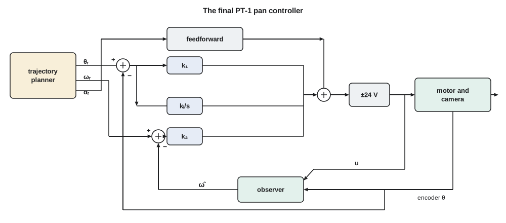
State feedback alone has the same weakness as the cascade: a constant disturbance leaves a steady error. The remedy is the same too, integral action, added as an extra state. Define z with ż = r − θ, the integral of the angle error, and feed it back: u = k₁(r − θ) − k₂ω + k_iz. The augmented system has three states and three closed-loop poles. For a first try Amara keeps the dominant pair at −20 ± j26.6 and places the third, the integrator's pole, at −25, just to the left of them, so that the integral action acts quickly. Matching the coefficients of s³ + (21 + 8.33k₂)s² + 8.33k₁s + 8.33k_i to (s² + 40s + 1108)(s + 25) gives the gains.
Observability and observers
State feedback needs the states, but the PT-1 measures only the angle. The speed must be estimated. Differencing successive encoder readings works but is noisy: one count in a millisecond is a speed of 0.063 rad/s, and the difference jumps by that much whenever the angle crosses a count. An observer does better. It runs a copy of the plant model in the controller, driven by the same input, and corrects the copy's states using the difference between the measured and predicted outputs: x̂̇ = Ax̂ + Bu + L(y − Cx̂). The estimation error then obeys ė = (A − LC)e, so the observer's gain L sets how fast the estimate converges.
The dual of controllability applies: the observer's poles, the eigenvalues of A − LC, can be placed anywhere if and only if the system is observable, which means the observability matrix [C; CA; …; CAⁿ⁻¹] has full rank. For the pan axis, measuring the angle makes both states observable. A common rule places the observer's poles three to ten times faster than the controller's, so that the estimate settles before it matters, but not so fast that the observer passes encoder noise straight through. Amara first puts both at −200 rad/s, ten times the controller's real part. Matching s² + (21 + l₁)s + (21l₁ + l₂) to (s + 200)² gives l₁ = 379 s⁻¹ and l₂ = 32 041 s⁻². The separation principle guarantees that, for a linear model, the controller and observer poles can be designed independently: the closed loop has exactly the poles of A − BK and A − LC. It says nothing about stability margins, which must be checked separately.
Trajectories and feedforward
Lessons 4, 8 and 10 noted that large steps saturate the driver. A step command asks for an instantaneous jump in angle, which no motor can deliver; the controller responds by commanding full voltage and the loop behaves nonlinearly. Motion-control systems therefore never command steps. A trajectory planner turns each move into a smooth reference with limited speed and acceleration. The simplest is the trapezoidal velocity profile: accelerate at a constant rate to a cruise speed, cruise, then decelerate, or, for a short move, accelerate and immediately decelerate in a triangular profile. Amara chooses a cruise speed of 150°/s and an acceleration of 1200°/s², which keep the voltage well inside the driver's range and the image blur acceptable to the operators.
With a planned trajectory, the controller knows not only where the camera should be but how fast it should be moving and accelerating. A feedforward term uses that knowledge directly. Inverting the plant model, the voltage needed to give acceleration α_r at speed ω_r is u_ff = (α_r + 21ω_r)/8.33. If the model were perfect, feedforward alone would make the camera follow the trajectory exactly and the feedback would only correct model errors and disturbances. Feedback and feedforward complement each other: feedforward provides speed of response to commands without raising loop gain, and feedback provides accuracy and disturbance rejection without needing a perfect model. This is the two-degree-of-freedom structure in its most effective form.
Margins with the observer in the loop
Pole placement guarantees the poles of the model, not robustness to everything the model leaves out. Amara therefore breaks the loop at the motor voltage, as Leo does on the bench, and computes the loop gain of the observer-based controller with the full plant, the 0.8 ms delay and the bracket mode of lesson 10. The first try fails Daniel's review criteria: a phase margin of only 41.8° at nominal parameters and 32.2° with the heated housing, with a crossover near 44 rad/s, twice that of the lead-lag. The high integral gain and the fast integrator pole push the crossover up, and the observer adds lag there.
She retunes in the direction lessons 8 and 10 suggest: more damping in the dominant pair, now −20 ± j17.6 (ζ = 0.75), a slower integrator pole at −4, and a faster observer at −300 rad/s, so that its lag at crossover is smaller. The new gains are k₁ = 104 V/rad, k₂ = 2.76 V/(rad/s), k_i = 341 V/(rad·s), l₁ = 579 s⁻¹ and l₂ = 77 841 s⁻². The code below computes both designs' margins. The final design has a phase margin of 60.3° and a gain margin of 12.1 dB at nominal parameters, 51.4° and 15.4 dB with the heated housing and 59.7° and 10.5 dB with a strong motor. The peak sensitivity, about 1.9 to 2.2, is set mainly by the lightly damped bracket mode and is the one number above the usual target; Daniel's request for a notch filter and a stiffer bracket addresses it.
The final simulation
Amara's final simulation includes everything the course has identified: the full motor model with its electrical pole, a controller running at 1 kHz on quantized encoder readings, the observer, the ±24 V limit with clamping anti-windup, and a 1.5 N·m wind gust applied 1.6 s after the start, once the camera has arrived. She compares raw steps with profiled moves, with and without feedforward, for a 10° and a 90° move.
import math, cmath
deg = math.pi / 180
# camera-side model x = [theta, omega]: theta' = omega, omega' = -21 omega + 8.33 (u - 0.8 Td)
a, bgain = 21.0, 8.33
# 1. controllability: the matrix (B, AB) has columns (0, 8.33) and (8.33, -175); its determinant is -8.33^2
print(f"det [B AB] = {-(bgain**2):.1f} (nonzero, so controllable)")
# 2. state feedback with integral action: u = k1 (r - theta) - k2 omega + ki z,  z' = r - theta
# closed loop: s^3 + (a + b k2) s^2 + b k1 s + b ki = (s^2 + 2 sig s + sig^2 + wd^2)(s + p3)
def place(sig, wd, p3, wo):
    c2, c0 = 2 * sig, sig**2 + wd**2
    k2 = (c2 + p3 - a) / bgain; k1 = (c0 + c2 * p3) / bgain; ki = c0 * p3 / bgain
    l1 = 2 * wo - a; l2 = wo**2 - a * l1          # observer poles at -wo, -wo
    return k1, k2, ki, l1, l2
def margins(L, wlo=0.05, whi=3000.0, n=6000):
    """Crossover, phase margin, worst gain margin over all phase crossings, and peak sensitivity."""
    ws = [wlo * (whi / wlo) ** (k / n) for k in range(n + 1)]
    ph, prev, data = 0.0, None, []
    for w in ws:
        v = L(1j * w); p = cmath.phase(v)
        if prev is not None:
            d = p - prev
            while d > math.pi: d -= 2 * math.pi
            while d < -math.pi: d += 2 * math.pi
            ph += d
        else: ph = p
        prev = p; data.append((w, abs(v), math.degrees(ph)))
    k = next(i for i, (w, m, p) in enumerate(data) if m < 1)
    lo, hi = data[k - 1][0], data[k][0]
    for _ in range(60):                                   # refine the gain crossover
        mid = math.sqrt(lo * hi)
        lo, hi = (mid, hi) if abs(L(1j * mid)) > 1 else (lo, mid)
    wc = lo; pm = 180 + data[k][2] + math.degrees(cmath.phase(L(1j * wc)) - cmath.phase(L(1j * data[k][0])))
    gm = min((-20 * math.log10(m2) for (w1, m1, p1), (w2, m2, p2) in zip(data, data[1:])
              if math.floor((p1 + 180) / 360) != math.floor((p2 + 180) / 360)), default=float('inf'))
    ms = max(1 / abs(1 + L(1j * w)) for w, _, _ in data)
    return wc, pm, gm, ms
def loop(gains, Jscale=1.0, kscale=1.0):
    """Loop gain broken at the motor voltage: observer-based controller, full plant, 0.8 ms delay, bracket mode."""
    k1, k2, ki, l1, l2 = gains
    def L(s):
        m11, m21, m22 = s + l1, l2, s + a                 # observer (sI - A + LC), off-diagonal -1
        det = m11 * m22 + m21
        Hu, Hy = m11 * bgain / det, (-m21 * l1 + m11 * l2) / det
        C = ((k1 + ki / s) + k2 * Hy) / (1 + k2 * Hu)
        G = kscale * 16667 / Jscale / (s * (s + 21.2 / Jscale) * (s + 1979))
        return C * G * cmath.exp(-0.8e-3 * s) * 260.0**2 / (s * s + 2 * 0.02 * 260.0 * s + 260.0**2)
    return L
first = place(20.0, 26.6, 25.0, 200.0)
final = place(20.0, 17.6, 4.0, 300.0)
for name, g in (("first try", first), ("final", final)):
    print(f"{name:9s}: k1 = {g[0]:5.1f} V/rad, k2 = {g[1]:.2f} V/(rad/s), ki = {g[2]:5.0f} V/(rad*s); observer l1 = {g[3]:.0f}, l2 = {g[4]:.0f}")
    for case, J, k in (("nominal", 1.0, 1.0), ("heated housing", 1.4, 1.0), ("strong motor", 1.0, 1.2)):
        wc, pm, gm, mx = margins(loop(g, J, k))
        print(f"   {case:15s} crossover {wc:5.1f} rad/s, PM {pm:4.1f} deg, GM {gm:4.1f} dB, peak |S| {mx:.2f}")
k1, k2, ki, l1, l2 = final
# 4. trapezoidal move profile with speed and acceleration limits
def profile(dist, vmax, amax):
    ta = vmax / amax; da = 0.5 * amax * ta**2
    if 2 * da > dist: ta = math.sqrt(dist / amax); vmax = amax * ta; da = dist / 2
    tc = (dist - 2 * da) / vmax; T = 2 * ta + tc
    def ref(t):
        if t <= 0: return 0.0, 0.0, 0.0
        if t < ta: return 0.5 * amax * t * t, amax * t, amax
        if t < ta + tc: return da + vmax * (t - ta), vmax, 0.0
        if t < T: d = T - t; return dist - 0.5 * amax * d * d, amax * d, -amax
        return dist, 0.0, 0.0
    return ref, T
# 5. full simulation: electrical pole, 1 kHz controller, encoder quantization, +-24 V limit, wind gust
R, L, Kt, J, b, N = 2.0, 1e-3, 0.05, 6e-5, 1e-5, 50
q = 2 * math.pi / 100000                                      # one encoder count at the camera
def run(use_profile, feedforward, dist_deg=90.0, t_end=4.0, gust=(1.6, 1.5)):
    dist = dist_deg * deg
    ref, T = profile(dist, 150 * deg, 1200 * deg) if use_profile else ((lambda t: (dist, 0.0, 0.0)), 0.0)
    i = wm = th = 0.0; th_h = w_h = z = 0.0; u = 0.0; t = 0.0; dt = 2e-5; k = 0
    worst_track, umax, imax, peak, last_out, gdev = 0.0, 0.0, 0.0, 0.0, 0.0, 0.0
    while t < t_end:
        if k % 50 == 0:                                           # controller at 1 kHz
            y = round(th / q) * q
            r, rd, rdd = ref(t)
            e_obs = y - th_h                                      # observer update (Euler, 1 ms)
            th_h, w_h = th_h + 1e-3 * (w_h + l1 * e_obs), w_h + 1e-3 * (-a * w_h + bgain * u + l2 * e_obs)
            z_new = z + 1e-3 * (r - y)
            uff = (rdd + a * rd) / bgain if feedforward else 0.0
            u_raw = k1 * (r - y) + k2 * (rd - w_h) + ki * z_new + uff
            u = max(-24.0, min(24.0, u_raw))
            if u == u_raw: z = z_new                              # clamping anti-windup
            umax = max(umax, abs(u))
            if 0.0 < t < T: worst_track = max(worst_track, abs(r - th))
        Td = gust[1] if t >= gust[0] else 0.0
        i += dt * (u - R * i - Kt * wm) / L
        wm += dt * (Kt * i - b * wm - Td / N) / J
        th += dt * wm / N; t += dt; k += 1
        imax = max(imax, abs(i)); peak = max(peak, th)
        if t >= gust[0]: gdev = max(gdev, abs(th - dist))
        if t < gust[0] and abs(th - dist) > 0.02 * dist: last_out = t
    return T, worst_track, umax, imax, (peak / dist - 1) * 100, last_out, gdev, th
cases = [("10 deg step, no profile", False, False, 10.0), ("10 deg profile + feedfwd", True, True, 10.0),
         ("90 deg step, no profile", False, False, 90.0),
         ("90 deg profile, feedback", True, False, 90.0), ("90 deg profile + feedfwd", True, True, 90.0)]
for name, prof, ff, d in cases:
    T, track, umax, imax, over, done, gdev, th = run(prof, ff, d)
    print(f"{name:25s}: move time {T:.3f} s, worst tracking error {track/deg:5.3f} deg, peak {umax:4.1f} V and {imax:4.1f} A, "
f"overshoot {over:4.1f} %, within 2 % from {done:.3f} s; gust pushes {gdev/deg:.3f} deg, {abs(th - d*deg)/deg:.4f} deg left at 4 s")det [B AB] = -69.4 (nonzero, so controllable) first try: k1 = 253.0 V/rad, k2 = 5.28 V/(rad/s), ki = 3324 V/(rad*s); observer l1 = 379, l2 = 32041 nominal crossover 43.5 rad/s, PM 41.8 deg, GM 10.7 dB, peak |S| 1.92 heated housing crossover 35.0 rad/s, PM 32.2 deg, GM 13.7 dB, peak |S| 1.81 strong motor crossover 50.9 rad/s, PM 42.0 deg, GM 9.1 dB, peak |S| 2.14 final : k1 = 104.4 V/rad, k2 = 2.76 V/(rad/s), ki = 341 V/(rad*s); observer l1 = 579, l2 = 77841 nominal crossover 27.3 rad/s, PM 60.3 deg, GM 12.1 dB, peak |S| 1.94 heated housing crossover 22.9 rad/s, PM 51.4 deg, GM 15.4 dB, peak |S| 1.59 strong motor crossover 31.8 rad/s, PM 59.7 deg, GM 10.5 dB, peak |S| 2.21 10 deg step, no profile : move time 0.000 s, worst tracking error 0.000 deg, peak 18.3 V and 8.6 A, overshoot 18.7 %, within 2 % from 0.660 s; gust pushes 0.694 deg, 0.0009 deg left at 4 s 10 deg profile + feedfwd : move time 0.183 s, worst tracking error 0.073 deg, peak 7.4 V and 1.3 A, overshoot 0.7 %, within 2 % from 0.162 s; gust pushes 0.696 deg, 0.0010 deg left at 4 s 90 deg step, no profile : move time 0.000 s, worst tracking error 0.000 deg, peak 24.0 V and 11.6 A, overshoot 4.1 %, within 2 % from 0.384 s; gust pushes 0.689 deg, 0.0018 deg left at 4 s 90 deg profile, feedback : move time 0.725 s, worst tracking error 3.617 deg, peak 8.3 V and 1.5 A, overshoot 3.7 %, within 2 % from 0.875 s; gust pushes 0.637 deg, 0.0017 deg left at 4 s 90 deg profile + feedfwd : move time 0.725 s, worst tracking error 0.057 deg, peak 9.1 V and 1.3 A, overshoot 0.1 %, within 2 % from 0.669 s; gust pushes 0.697 deg, 0.0017 deg left at 4 s
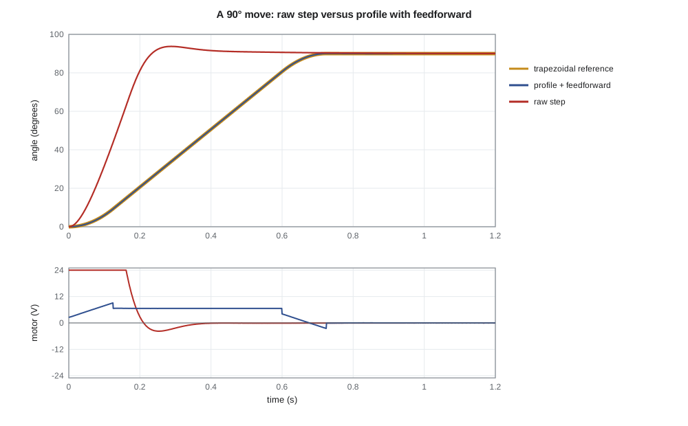
The raw 10° step shows why steps are a poor idea with an integral state-feedback controller: the error enters k₁ and the integrator at once, the motor jumps to 18.3 V and 8.6 A, the camera overshoots by 18.7 % and the slow integrator pole keeps it outside the 2 % band until 0.66 s. The same move made through the planner, a triangular profile of 0.183 s, peaks at 7.4 V and 1.3 A, overshoots by only 0.7 % and is within 2 % from 0.16 s. It meets lesson 1's transient specification with room to spare.
For the 90° move the contrast is sharper. The raw step pins the driver at 24 V and draws 11.6 A, overshoots by 4.1 %, about 3.7°, and is within 2 % only from 0.38 s. The profiled move takes 0.725 s, never needs more than 9.1 V or 1.3 A, and arrives cleanly. Without feedforward, the more gently tuned feedback lags the moving reference by up to 3.6° during the cruise and overshoots by 3.7 %; with feedforward the worst tracking error falls to 0.057°, more than sixty times smaller, and the overshoot to 0.1 %, with almost the same voltage. Feedforward lets the feedback be tuned for robustness without giving up tracking. The sudden 1.5 N·m gust pushes the camera about 0.7° off target, and the integral action brings it back to within 0.002°, about half an encoder count, by the end of the run. The ramp specification of lesson 1, 0.2° at 20°/s, is met by a wide margin, because the profile's cruise at 150°/s is tracked to within 0.06°.
Verification against the specification
| Specification (lesson 1) | Requirement | Final design |
|---|---|---|
| Small-move settling | ≤ 0.25 s to 2 % for 10° | 0.16 s (profiled) |
| Overshoot | ≤ 10 % | 0.5 % for 10°, 0 % for 90° |
| Tracking a pan | ≤ 0.2° at 20°/s | 0.057° worst case at 150°/s |
| Wind torque | Zero steady error | 0.7° transient, then within 0.002° |
| Robustness | PM ≥ 50°, GM ≥ 10 dB | PM 51°–60°, GM 10.5–15 dB over the parameter spread |
| Hardware limits | ±24 V, 1 kHz | Peak 9.1 V on 90° moves; 1 kHz with 0.8 ms delay modeled |
Daniel's final review asks for three things before release. First, the notch filter and stiffer bracket of lesson 10, to bring the peak sensitivity down and remove the dependence on phase stabilization. Second, field data: Leo installs two prototypes on a mast arm at Cedarline's test intersection and logs a week of moves, gusts and temperatures, including the heated housing on cold nights, and compares the measured loop response with the model. Third, documentation of every parameter that a production change, a new camera or a new gearbox, would affect, so that the next engineer knows which gains to revisit.
Worked problem
Pole placement for the tilt axis
The tilt axis, with states angle and speed, has ẋ = [0 1; 0 −15]x + [0; 5.0]u (ignoring its fast pole). Find state-feedback gains that place the closed-loop poles at −16 ± j15.4 (lesson 4), and an observer gain for observer poles at −160, −160 from an angle measurement.
Show solution
- Closed loop: s² + (15 + 5.0k₂)s + 5.0k₁. Desired: (s + 16)² + 15.4² = s² + 32s + 493.2.
- \[k_2 = \frac{32 - 15}{5.0} = 3.40\ \tfrac{\text{V}}{\text{rad/s}} \qquad k_1 = \frac{493.2}{5.0} = 98.6\ \tfrac{\text{V}}{\text{rad}}\]
- Observer: A − LC = [−l₁ 1; −l₂ −15], with characteristic polynomial s² + (15 + l₁)s + (15l₁ + l₂).
- \[15 + l_1 = 320 \Rightarrow l_1 = 305 \qquad 15 \times 305 + l_2 = 25\,600 \Rightarrow l_2 = 21\,025\]
Answer: K = [98.6 3.40] and L = [305; 21 025]. By the separation principle the closed loop has poles at −16 ± j15.4 and −160, −160.
Where to go next
This course has covered the classical core of control engineering and opened the door to state space. Beyond it lie several large fields. Digital control treats sampled systems directly in the z-domain, designing for the sampling rather than approximating it. Optimal control and estimation, the linear-quadratic regulator and the Kalman filter, choose gains by minimizing cost functions and handle noise statistically. Robust control, including H-infinity methods, designs for guaranteed performance across a range of plant models. Nonlinear control deals with saturation, friction and large motions directly. Model predictive control, now common in process plants and increasingly in power electronics and vehicles, solves an optimization at every sample to respect actuator and state limits explicitly. Each builds on the ideas here: models, feedback, poles, margins and the trade-offs between speed, accuracy, effort and robustness.
Common mistakes
MistakeCommanding steps to a high-gain servo.
InsteadUse a trajectory planner with speed and acceleration limits, and feedforward from the planned motion.
MistakeDifferencing a coarse encoder to get speed for state feedback.
InsteadUse an observer, with poles a few times faster than the controller's.
MistakeAssuming the separation principle preserves stability margins.
InsteadIt preserves pole locations, not margins; check the loop with the observer included.
MistakeRelying on feedforward without feedback.
InsteadFeedforward cannot correct model errors or disturbances; keep the feedback loop.
Summary and key terms
- A state-space model ẋ = Ax + Bu, y = Cx + Du describes internal states; the eigenvalues of A are the poles.
- If the system is controllable, state feedback u = −Kx places all closed-loop poles; position-plus-rate feedback is state feedback.
- Integral action is added as an extra state; an observer estimates unmeasured states, and the separation principle lets controller and observer poles be placed separately.
- Pole placement does not guarantee margins: the first pan design, with an integrator pole at −25 and observer at −200, had only 42° of phase margin.
- The final pan design places poles at −20 ± j17.6 and −4 with an observer at −300 (k₁ = 104, k₂ = 2.76, k_i = 341) and keeps 51° to 60° of phase margin over the parameter spread.
- A trapezoidal trajectory with feedforward keeps the 90° move within 9.1 V and tracks it to 0.057°, compared with 24 V saturation and 4.1 % overshoot for a raw step.
- The final design meets every lesson 1 specification; feedforward lets the feedback be tuned for robustness without losing tracking accuracy.
- State-space model
- First-order matrix differential equations ẋ = Ax + Bu, y = Cx + Du.
- Controllability
- The ability of the input to drive the state anywhere; full rank of [B AB … Aⁿ⁻¹B].
- Observability
- The ability to determine the state from the output; full rank of [C; CA; …; CAⁿ⁻¹].
- State feedback
- A control law u = −Kx + k_r r using all the states.
- Pole placement
- Choosing feedback gains to put closed-loop poles at specified locations.
- Observer
- A model-based estimator x̂̇ = Ax̂ + Bu + L(y − Cx̂) for unmeasured states.
- Separation principle
- For linear systems, controller and observer poles can be designed independently.
- Feedforward
- A control signal computed from the reference, without feedback, to speed tracking.
Practice problems
Work each problem on paper first, then reveal the answer to check.
Write the state equations of 1/(s(s + 4)) with states angle and speed.
Show answer
ẋ = [0 1; 0 −4]x + [0; 1]u, y = [1 0]x.
Is the pair A = [0 1; 0 −4], B = [1; 0] controllable?
Show answer
[B AB] = [1 0; 0 0] has rank 1: not controllable, since the input does not reach the speed.
For the pan plant, what k₁ and k₂ place the poles at −30 ± j30?
Show answer
s² + 60s + 1800: k₂ = 39/8.33 = 4.68, k₁ = 1800/8.33 = 216.
What feedforward voltage does a 150°/s cruise need?
Show answer
u_ff = 21 × 2.62/8.33 = 6.6 V.
How long is a triangular profile for a 10° move with 1200°/s² acceleration?
Show answer
t_a = √(10/1200) = 0.091 s, so 0.183 s in total.
Why are observer poles placed faster than controller poles but not arbitrarily fast?
Show answer
So the estimate converges before it matters, without amplifying measurement noise.
Lesson quiz · 5 questions
Score 60% or more to complete this lesson.
Create a free account to save your progress, take quizzes and earn a certificate.