High-performance and AI cluster networks

Training a large AI model is one enormous calculation spread across thousands, sometimes hundreds of thousands, of accelerators. No single chip has enough memory or speed, so the model and the data are divided among them, and the accelerators must constantly exchange results. If the network cannot keep up, the most expensive computers ever built sit idle, waiting. In an AI training cluster the network is not a supporting system; it is part of the computer.

High-performance computing (HPC) clusters for science and engineering have faced the same problem for decades, and AI networks borrow much from them. This chapter explains why AI training is so demanding on the network, the three networks inside an AI cluster, the technologies used (NVLink and other scale-up links, InfiniBand, and RDMA over Ethernet), how cluster fabrics are built and sized, and what all this means for the data center: thousands of optics, enormous fiber counts, high power and tight distance limits.

Why AI training stresses the network

A neural network is trained in steps. In each step, a batch of training examples flows forward through the model, the error is measured, and gradients (the direction in which each parameter should change) flow backward. Then every parameter is updated. A large model has hundreds of billions of parameters.

The simplest way to use many accelerators is data parallelism: every accelerator holds a full copy of the model and processes a different slice of the batch. After the backward pass, each accelerator has its own gradients, and they must be averaged across all accelerators before anyone can update the model. That averaging is a collective operation called all-reduce, and every accelerator must finish it before the next step begins. Larger models also split the model itself across accelerators, using tensor parallelism (splitting individual layers), pipeline parallelism (placing different layers on different accelerators) and expert parallelism (spreading the "experts" of a mixture-of-experts model), each with its own communication pattern.

Three features make this traffic unlike ordinary data center traffic:

• It is synchronized. Thousands of accelerators finish computing at the same moment and then all transmit at full speed at once. There is no statistical smoothing of the kind that justifies oversubscription in a general-purpose fabric.
• It is made of huge flows. Gradients are gigabytes, sent between the same pairs of accelerators again and again. These elephant flows defeat the hash-based load balancing described in Lesson 3.
• The slowest link sets the pace. A collective finishes only when the last accelerator finishes. One congested link, one failing optic or one slow switch port delays the entire job. Engineers talk about tail latency and job completion time rather than average throughput.

In a well-designed cluster, communication overlaps with computation and takes a modest share of each step. In a poorly designed one, accelerators may spend a large fraction of their time waiting, which on a cluster costing billions of dollars is an enormous waste.

The ring all-reduce

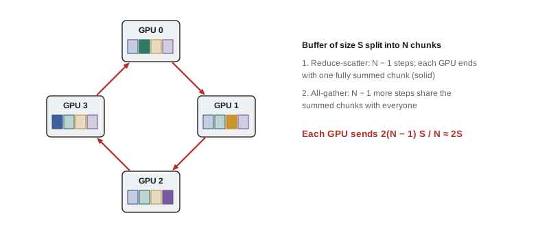
A classic way to perform an all-reduce among \(N\) accelerators is to arrange them in a logical ring. The gradient buffer of size \(S\) is split into \(N\) chunks. In the first phase (reduce-scatter), each accelerator repeatedly sends one chunk to its neighbor and adds the chunk it receives, so after \(N-1\) steps each accelerator holds one fully summed chunk. In the second phase (all-gather), the summed chunks travel around the ring for another \(N-1\) steps until everyone has all of them. Each accelerator sends a total of:

For large \(N\) this approaches \(2S\): each accelerator sends about twice the size of the gradients, almost regardless of how many accelerators there are. The time is roughly \(D\) divided by each accelerator's network bandwidth, plus latency for each of the \(2(N-1)\) steps. Real libraries such as NCCL use rings, trees and hierarchical schemes chosen to suit the topology, but the ring shows the key point: the bandwidth per accelerator directly sets the communication time.

The three networks of an AI cluster

A modern AI cluster has three distinct networks, each with its own purpose, technology and cabling:

• The scale-up network connects a small group of accelerators so tightly that they behave almost like one large accelerator with shared memory. It runs at very high bandwidth and very low latency over short distances, usually within a server or a rack. Examples are NVIDIA's NVLink, AMD's Infinity Fabric and the open UALink standard (version 1.0 published in 2025). In a rack-scale system such as NVIDIA's GB200 NVL72, NVLink switches connect 72 GPUs, each with about 1.8 TB/s of total NVLink bandwidth, over thousands of short copper cables in the rack spine. A single rack like this can draw about 120 kW or more and needs liquid cooling.
• The scale-out or back-end network connects the scale-up domains to each other across the cluster. Each accelerator usually has its own network adapter at 400 or 800 Gb/s. This is the large, non-blocking fabric this chapter focuses on, built with InfiniBand or with Ethernet tuned for AI.
• The front-end network connects the cluster to storage, to the rest of the data center, to users and to the internet. It carries training data in, model checkpoints out to storage, and management traffic. It is a conventional leaf-spine Ethernet fabric (Lesson 3), typically with oversubscription and lower bandwidth per server than the back-end.

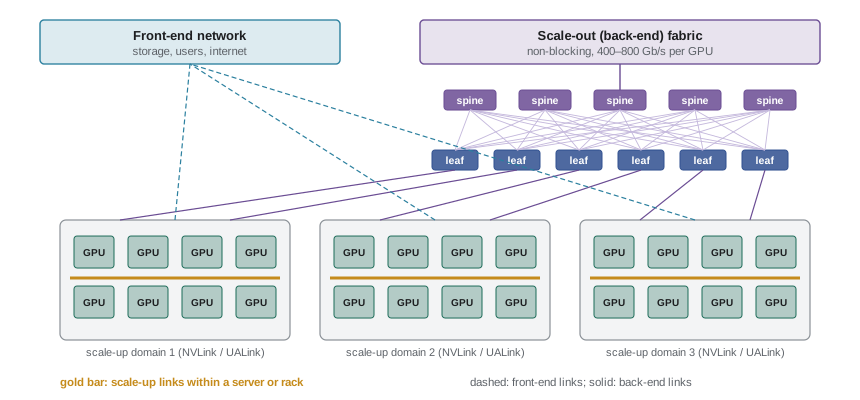
A separate out-of-band management network, as in Lesson 1, connects every server's management controller, switch and power distribution unit, bringing the total to four.

Scale-out technologies: InfiniBand and Ethernet

RDMA

Ordinary networking passes data through the operating system: the application copies data into kernel buffers, the TCP stack processes it, and the network card sends it, with the reverse at the other end. This costs CPU time and adds latency. Remote direct memory access (RDMA) lets a network adapter read from or write into the memory of a remote machine directly, bypassing the operating system and the CPU on both sides. With GPUDirect RDMA, the adapter reads and writes GPU memory directly, so gradients go from one accelerator's memory to another's with no copies through host memory. Every AI back-end network uses RDMA.

InfiniBand

InfiniBand is a networking technology designed from the start for HPC. It has its own switches, adapters and protocols, controlled by a central subnet manager that computes routes for the whole fabric. Its key feature is credit-based, lossless flow control: a sender transmits only when the receiver has advertised buffer space, so packets are never dropped because of congestion. Current generations are NDR (400 Gb/s per port) and XDR (800 Gb/s). InfiniBand switches can also perform some collective operations inside the network, reducing the data the accelerators must exchange. InfiniBand has long dominated the largest AI training clusters, and it is supplied mainly by one vendor.

Ethernet for AI: RoCE and Ultra Ethernet

Ethernet has many suppliers, a huge ecosystem and the operational familiarity of every data center team, and it now carries a large and growing share of AI back-end networks. RDMA runs over Ethernet using RoCE v2 (RDMA over Converged Ethernet), which places RDMA traffic inside UDP/IP packets so it can be routed across a leaf-spine fabric.

The challenge is that RDMA performs badly when packets are lost, and ordinary Ethernet drops packets when buffers overflow. AI Ethernet fabrics address this with:

• Priority Flow Control (PFC, IEEE 802.1Qbb), which lets a switch tell its neighbor to pause one class of traffic briefly when its buffers fill, making that class lossless.
• Explicit Congestion Notification (ECN), in which switches mark packets when queues start to build, and the endpoints slow down before losses occur.
• Advanced load balancing: spraying packets of a flow across many paths, or adaptive routing that steers traffic around congested links, instead of the static per-flow ECMP hash that elephant flows defeat.

The Ultra Ethernet Consortium, an industry group, published version 1.0 of its specification in 2025, defining a new transport designed for AI and HPC over Ethernet with multipath packet spraying, modern congestion control and tolerance of out-of-order delivery, aiming to deliver InfiniBand-class performance on standard Ethernet hardware.

Building the back-end fabric

Fat trees and non-blocking design

AI back-end fabrics are Clos networks like those in Lesson 3, but built non-blocking (1:1) at every layer. In the HPC world, a non-blocking Clos network is often called a fat tree, because the bandwidth stays the same (the branches stay "fat") all the way to the top. With switches of radix \(k\) (ports per switch), each leaf uses half its ports for accelerators and half for uplinks. A two-tier non-blocking fat tree supports:

and a three-tier fat tree supports:

Switch radix therefore matters enormously. Doubling the radix quadruples the size of a two-tier fabric and multiplies a three-tier fabric by eight, while each extra tier adds switches, optics, latency and cost. This is why switch vendors push for higher radix as hard as for higher speed, and why a 51.2 Tb/s switch is often run as 128 ports of 400 Gb/s rather than 64 of 800 Gb/s in AI fabrics.

Rail-optimized topology

AI servers typically hold eight accelerators, each with its own network adapter. In a rail-optimized design, accelerator number 0 in every server connects to one set of leaf switches (rail 0), accelerator 1 in every server to rail 1, and so on, up to rail 7. Communication libraries arrange collectives so that most traffic passes between accelerators with the same index in different servers, which then needs only one hop through a rail leaf. Traffic between different indices moves first across the fast NVLink inside the server and then along the right rail. Rail-optimized designs reduce the load on the spine layer and the latency of the most common transfers.

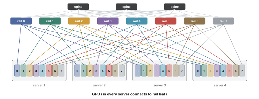
Rail designs have a physical consequence: each server sends eight cables to eight different leaf switches, often in a different rack, rather than to one top-of-rack switch. Leaves for a group of GPU racks are usually placed together in network racks at the end or middle of the rows, and every GPU rack has dozens of fibers running to them.

What AI networks mean for the facility

AI clusters change the data center design brief in ways that land directly on the facility engineer:

• Distance limits shape the floor plan. Copper scale-up links reach only a couple of meters, which is why scale-up domains are built as single racks or adjacent racks. Back-end optics have reach limits too, and latency adds up with fiber length (about 5 ns per meter). Designers lay out GPU racks, network racks and spines to keep every run within the reach of the chosen optics, often arranging a cluster as compact "pods" or "scalable units" with the network at the center.
• Fiber counts are enormous. A cluster of tens of thousands of GPUs can have hundreds of thousands of fiber terminations. Overhead tray capacity, patch panels and installation labor become major cost and schedule items, and pre-terminated MPO trunks and high-count ribbon cables are standard.
• Network power and cooling are substantial. Switches and optics can add several percent to the IT load, network racks may draw 20 to 40 kW, and some new switch platforms are liquid cooled like the accelerators.
• Rack density changes everything else. Scale-up racks at 100 kW and above require direct-to-chip liquid cooling (DCE-330), heavy power distribution (DCE-310) and floors or slabs rated for racks weighing well over a metric ton (DCE-430).
• Reliability is about the job, not the link. Because one failed link can stall a training job across thousands of accelerators, operators monitor every optic, keep spares on site and design for fast replacement. Optics, and especially the dust on their connectors, are among the most common failure points in a cluster.
• Storage and checkpoints need their own bandwidth. Training jobs periodically save checkpoints, the full model and optimizer state, so they can restart after a failure. These bursts travel over the front-end or a dedicated storage network.

Beyond training

Inference (running trained models to answer requests) is a growing share of AI computing. A single inference request usually runs within one server or one scale-up domain, so inference clusters need less back-end bandwidth than training clusters and rely more on the front-end network and on latency to users. Large models served at scale still split work across accelerators, however, and newer serving designs move intermediate results between separate groups of accelerators, so inference fabrics are becoming more demanding too.

At the other extreme, the largest training efforts are now spreading across multiple buildings and even multiple campuses, linked by massive DWDM systems (Lesson 9) carrying hundreds of terabits per second between sites. Distributing training across sites hundreds of kilometers apart brings the latency limits of Lesson 7 into the design of the training software itself.