
CON-310 · Lesson 8 of 12 · 24 min
Earned value analysis and earned schedule
Lesson 7 defined the earned value measures. This lesson is about using them: reading trends rather than single values, converting schedule variance from dollars into time with earned schedule, setting variance thresholds, writing variance analysis that leads to action, and knowing the limits of the method. The aim is to get from 'the SPI is 0.89' to 'the structure is about three weeks behind because slab forming on level 3 is running at 85 % of budget productivity, and here is what we are doing about it.'
Trends, not snapshots
A single month's CPI or SPI says little on its own. A CPI of 0.97 might be improving from 0.90 or deteriorating from 1.05; the response should be very different. Earned value reports should therefore show both cumulative and current-period indices over time. Cumulative indices are stable and show the overall position; period indices are noisy but show what is happening now. When the period index stays below the cumulative one for several months, the cumulative index will keep falling.
# Cumulative and monthly CPI for the Riverbend structure account (amounts $1000)
ev = [0, 180, 640, 1_210, 1_820, 2_330, 2_780]      # cumulative earned value, months 2-8
ac = [0, 176, 655, 1_265, 1_915, 2_480, 2_960]      # cumulative actual cost
for m in range(1, len(ev)):
    month_cpi = (ev[m] - ev[m - 1]) / (ac[m] - ac[m - 1])
print(f"Month {m + 2}: monthly CPI {month_cpi:.2f} cumulative CPI {ev[m] / ac[m]:.3f}")Month 3: monthly CPI 1.02 cumulative CPI 1.023 Month 4: monthly CPI 0.96 cumulative CPI 0.977 Month 5: monthly CPI 0.93 cumulative CPI 0.957 Month 6: monthly CPI 0.94 cumulative CPI 0.950 Month 7: monthly CPI 0.90 cumulative CPI 0.940 Month 8: monthly CPI 0.94 cumulative CPI 0.939
The monthly CPI fell below 1.0 in month 4 and has stayed there, between about 0.90 and 0.96. The cumulative CPI therefore keeps drifting down. Nothing in the trend suggests a recovery without action.
How stable is the CPI?
Research on large defense contracts in the United States, notably by David Christensen and colleagues in the 1990s, found that once a contract was about 20 % complete, its cumulative CPI rarely changed by more than about 10 % for the rest of the contract, and when it did change it usually got worse. Construction projects are less studied and differ in many ways, so the finding should be treated as a caution rather than a law. But the practical message is consistent with experience on building projects: early cost performance is a strong predictor of the final result, and a project manager who expects a poor cumulative CPI to recover by itself is usually disappointed. Lesson 9 uses this when choosing forecasting formulas.
The problem with SV in dollars
Schedule variance in dollars has a well-known flaw. At the end of a project, all the work is done, so earned value equals planned value equals BAC, and SV returns to zero and SPI to 1.0, even if the project finished months late. In the last third of a late project, SV and SPI drift back toward 'on schedule' and become misleading. They also say nothing directly about time: being $953,000 of work behind does not tell anyone how many weeks late the project is.
Earned schedule
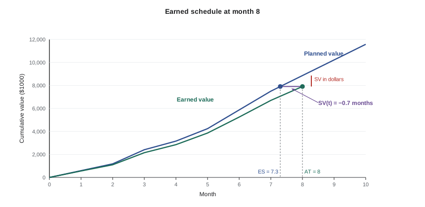
Earned schedule (ES), introduced by Walt Lipke in 2003, fixes the problem by measuring schedule performance in time. ES is the time at which the planned value curve reached the current earned value: in other words, how far along the baseline the project has actually got. It is found by locating the period in which PV passed EV and interpolating within it.
Here \(C\) is the number of whole periods for which cumulative PV is less than or equal to EV, \(PV_C\) is cumulative PV at the end of period \(C\), and \(PV_{C+1}\) at the end of the next period. With ES and the actual time elapsed (AT), schedule variance and performance can be expressed in time.
# Earned schedule for Riverbend Commons at month 8 (amounts $1000)
pv = [0, 592, 1_185, 2_409, 3_160, 4_242, 5_872, 7_502, 8_860, 10_218, 11_576]   # cumulative PV, months 0-10
EV, AT, PD = 7_907, 8, 16          # earned value, actual time (months), planned duration
C = max(m for m in range(len(pv)) if pv[m] <= EV)
ES = C + (EV - pv[C]) / (pv[C + 1] - pv[C])
sv_t, spi_t = ES - AT, ES / AT
print(f"C = {C}; ES = {ES:.2f} months")
print(f"SV(t) = {sv_t:.2f} months ({sv_t * 4.33:.1f} weeks); SPI(t) = {spi_t:.3f}")
print(f"Dollar SPI for comparison: {EV / pv[AT]:.3f}")
print(f"Forecast duration at SPI(t): {PD / spi_t:.1f} months")C = 7; ES = 7.30 months SV(t) = -0.70 months (-3.0 weeks); SPI(t) = 0.912 Dollar SPI for comparison: 0.892 Forecast duration at SPI(t): 17.5 months
Riverbend Commons has achieved the planned value of month 7.3 by month 8, so it is about 0.7 months, or roughly three weeks, behind. If performance continues at SPI(t) = 0.912, the 16-month job would take about 17.5 months. That is a little worse than the 17 months the project team used for its general conditions forecast in Lesson 6, which is exactly the kind of difference the monthly review should discuss.
Worked problem
Why SPI(t) is better late in the job
A 12-month project finishes in month 15. At month 14, EV is $9.85 million against BAC of $10 million, and PV has been $10 million since month 12. Compare the dollar SPI with SPI(t), where the baseline PV reached $9.85 million at month 11.6.
Show solution
- Dollar SPI = 9.85 ÷ 10.00 = 0.985: it looks almost on schedule.
- ES = 11.6 months; AT = 14 months.
- SPI(t) = 11.6 ÷ 14 = 0.83; SV(t) = −2.4 months.
Answer: The dollar SPI says the job is 98.5 % on schedule; SPI(t) correctly shows it is running at 83 % of planned pace and is 2.4 months behind.
Earned value and the critical path
Earned value, including earned schedule, measures progress across all work, weighted by budget. The project's completion date, however, depends on the critical path (CON-210 Lesson 5). A project can show SPI(t) close to 1.0 because non-critical work is ahead, while the critical path is slipping; or it can show a poor SPI because non-critical work is behind, with no effect on the end date. Earned schedule is therefore a useful independent check on the scheduler's forecast, not a replacement for it. When the two disagree, look at the critical and near-critical activities: if they are behind, believe the worse figure.
Variance thresholds
No team can investigate every variance every month. Thresholds focus attention on the ones that matter. A typical approach sets thresholds on both percentage and absolute value, so that small accounts are not flagged for trivial amounts and large accounts are not let off because the percentage is small.
| Measure | Report required if | Example threshold |
|---|---|---|
| Cumulative CV | Beyond ± percentage of EV and ± absolute amount | ± 5 % and ± $25,000 |
| Cumulative SV or SV(t) | Beyond ± percentage of PV or ± time | ± 10 % or ± 2 weeks |
| Variance at completion (Lesson 9) | Beyond ± percentage of BAC | ± 3 % |
| Change in forecast since last month | Beyond an absolute amount | ± $15,000 |
# Flag control accounts that breach thresholds (amounts $1000)
accounts = {  # name: (PV, EV, AC)
    "Site and foundations": (1_420, 1_420, 1_455), "Structure": (3_160, 2_780, 2_960),
    "Envelope": (1_644, 1_370, 1_390), "Mechanical and electrical": (1_324, 1_210, 1_200),
    "Interiors": (360, 175, 180), "General conditions": (952, 952, 978),
}
for name, (pv, ev, ac) in accounts.items():
    cv, sv = ev - ac, ev - pv
    flags = []
    if abs(cv) > 25 and abs(cv) / ev > 0.05: flags.append(f"CV {cv:+}")
    if abs(sv) / pv > 0.10: flags.append(f"SV {sv:+}")
print(f"{name:<27} {'; '.join(flags) if flags else 'within thresholds'}")Site and foundations within thresholds Structure CV -180; SV -380 Envelope SV -274 Mechanical and electrical within thresholds Interiors SV -185 General conditions within thresholds
Structure breaches both cost and schedule thresholds. Envelope and interiors breach the schedule threshold. General conditions' CV of minus $26,000 is above the absolute amount but under 5 % of EV, so it is not flagged; it will be caught by the forecast change threshold if the overrun grows. Site and foundations is slightly over on cost but within both limits.
Variance analysis that leads to action
For each breach, the control account manager writes a short variance analysis. A good one answers four questions in plain language: what is the variance; what caused it; what will its impact be on cost and schedule at completion; and what is being done about it, by whom and by when. A poor one restates the numbers ('CV is −$180,000 because actual cost exceeded earned value') or blames the weather without evidence.
| Element | Weak example | Strong example |
|---|---|---|
| Variance | Structure is over budget | Structure CV −$180,000 (CPI 0.94); SV(t) about −3 weeks |
| Cause | Productivity issues | Level 2 and 3 elevated slab forming ran at PF 0.82 because the shoring layout drawings were late and crews re-laid shoring twice; two cold weeks added heating and slowed placing |
| Impact | May overrun | If level 4 and roof run at PF 0.92, structure finishes about $245,000 over and 3 weeks late, delaying envelope start by 2 weeks |
| Corrective action | Will monitor | Shoring drawings for level 4 and roof approved; added an experienced forming foreman; second shift for strip and reshore on level 4; review weekly PF on Fridays (superintendent) |
Using earned value in the weekly meeting
On self-performed work, the most useful earned value conversation happens weekly at crew level, in hours. A one-page sheet for each foreman showing budget hours, earned hours, actual hours, weekly and cumulative productivity factor, and the hours remaining at the current rate makes the numbers concrete. Crews that see their own figures every week, and are asked what is getting in their way, often identify the problems faster than any analyst: late drawings, missing materials, crane conflicts, an inspection backlog. The cost engineer's job is to make the numbers accurate and simple enough for that conversation.
Limits of earned value
Earned value is a powerful summary but it has limits. It measures performance against the baseline, so a bad baseline gives bad answers. It weights work by budget, so a cheap but critical activity has little influence on SPI. It says nothing about quality: work that will need rework has still been 'earned' unless the rules of credit remove it. And it depends on honest progress measurement, the step most open to optimism. Used with these limits in mind, alongside the schedule and the line-by-line cost forecast, it is the best early warning system a project has.
Common mistakes
MistakeReacting to a single month's index.
InsteadLook at cumulative and period indices over several months.
MistakeExpecting a poor cumulative CPI to recover without action.
InsteadTreat early cost performance as a strong predictor and act on the cause.
MistakeReading dollar SV late in a project as a measure of lateness.
InsteadUse earned schedule: SV(t) and SPI(t) remain valid to the end.
MistakeTrusting SPI(t) over the critical path analysis.
InsteadUse earned schedule as a check; the critical path decides the end date.
MistakeWriting variance analysis that restates the numbers.
InsteadState the cause, the impact at completion and specific corrective actions with owners and dates.
MistakeKeeping earned value in the office.
InsteadShare hours-based figures with foremen weekly and ask what is getting in their way.
Summary and key terms
- Read cumulative and period indices together; trends matter more than snapshots.
- Research on defense contracts suggests cumulative CPI rarely improves much after about 20 % completion.
- Dollar SV and SPI return to on-schedule values at completion and do not measure time.
- Earned schedule finds the time at which PV equalled current EV and gives SV(t) and SPI(t) in time units.
- Earned schedule checks, but does not replace, critical path analysis.
- Thresholds on percentage and absolute value focus attention on significant variances.
- Good variance analysis states cause, impact at completion and corrective actions with owners.
- Cumulative index
- An index calculated from cumulative values since the start.
- Period index
- An index calculated from the values for the current period only.
- Earned schedule (ES)
- The time at which planned value reached the current earned value.
- Actual time (AT)
- The time elapsed from the start to the status date.
- SV(t)
- Schedule variance in time: ES minus AT.
- SPI(t)
- Schedule performance index in time: ES divided by AT.
- Variance threshold
- A limit beyond which a variance must be analyzed and reported.
- Variance analysis
- A written explanation of a variance's cause, impact and corrective action.
- Control account manager
- The person responsible for a control account's scope, schedule and cost.
- CPI stability
- The tendency of cumulative CPI to change little after early in a project.
Practice problems
Work each problem on paper first, then reveal the answer to check.
Monthly CPI has been 0.88, 0.85 and 0.90 for three months, and cumulative CPI is 0.95. What will happen to the cumulative CPI?
Show answer
It will keep falling while monthly CPI stays below it.
Why does dollar SPI equal 1.0 at completion?
Show answer
All work is done, so EV equals PV equals BAC.
PV at month 5 is $2.0 million and at month 6 $2.6 million. EV at month 7 is $2.3 million. What is ES?
Show answer
5 + (2.3 − 2.0) ÷ (2.6 − 2.0) = 5.5 months.
Using that ES, what are SV(t) and SPI(t) at month 7?
Show answer
SV(t) = −1.5 months; SPI(t) = 0.786.
A 20-month project has SPI(t) = 0.90. What duration does it forecast?
Show answer
About 22.2 months.
Why might SPI(t) look good while the project is late?
Show answer
Non-critical work may be ahead while the critical path slips.
Why use both percentage and absolute thresholds?
Show answer
So small accounts are not flagged for trivial amounts and large accounts are not excused by small percentages.
Name the four elements of a good variance analysis.
Show answer
Variance, cause, impact at completion, corrective action with owner and date.
What is weak about 'CV is negative because actual cost exceeded earned value'?
Show answer
It restates the definition without a cause or action.
Give two limits of earned value.
Show answer
Depends on baseline quality, weights by budget not criticality, ignores quality, depends on honest progress.
Lesson quiz · 5 questions
Score 60% or more to complete this lesson.
Create a free account to save your progress, take quizzes and earn a certificate.