Randomized algorithms and hashing

A randomized algorithm makes some of its choices by flipping coins. That sounds like an admission of defeat, but randomness is one of the most effective tools in algorithm design. It defeats adversarial inputs that would make a deterministic algorithm slow, it makes simple algorithms fast on average for every input rather than for typical inputs only, and it allows tiny data structures that answer questions about enormous data sets with a controlled chance of error. This lesson examines randomized quicksort and quickselect, explains why universal hashing guarantees good average behavior, and introduces two probabilistic data structures that Northway uses: Bloom filters and reservoir sampling.

Two kinds of randomized algorithm are distinguished by what is random. A Las Vegas algorithm always gives the correct answer, and only its running time is random; randomized quicksort is an example. A Monte Carlo algorithm always finishes within a fixed time, and its answer is correct with high probability; the Miller-Rabin primality test used in key generation is an example. A Las Vegas algorithm can be turned into a Monte Carlo one by stopping it after a time limit, and a Monte Carlo algorithm whose answers can be checked cheaply can be turned into a Las Vegas one by repeating it until a check passes.

Expected running time

For a randomized algorithm, the running time on a fixed input is a random variable, and we analyze its expected value, then take the worst case over inputs. This is different from average-case analysis of a deterministic algorithm, which assumes the inputs themselves are random. Expected worst-case analysis makes no assumption about the input: an adversary may choose the worst input, but cannot predict the coin flips. Linearity of expectation, the fact that the expected value of a sum is the sum of the expected values even when the terms are dependent, is the workhorse of these analyses.

Randomized quicksort

Quicksort picks a pivot, partitions the array into elements smaller and larger than the pivot, and sorts the two parts recursively. With the first element as pivot, an already-sorted array, which is exactly what Northway's nodes upload most nights, makes every partition maximally unbalanced and the running time Θ(n²). Choosing the pivot uniformly at random makes the expected running time Θ(n log n) on every input.

The proof counts comparisons. Let the elements in sorted order be z₁ < z₂ < … < z_n, and let X_ij be 1 if z_i and z_j are ever compared. They are compared exactly when one of them is the first pivot chosen from the range z_i to z_j; if any element strictly between them is chosen first, they go to different sides and are never compared. The range has j − i + 1 elements, each equally likely to be first, so the probability is 2/(j − i + 1). Summing over all pairs gives about 2n ln n comparisons, roughly 1.39 n log₂ n.

Quickselect and the median

Dana's speed reports need the median vehicle speed at each site for each hour, and the 85th percentile, which traffic engineers use to set speed limits. Sorting each hour's speeds costs Θ(n log n). Quickselect finds the k-th smallest element in expected linear time by partitioning around a random pivot and recursing into only the side that contains position k. Because only one side is pursued, the expected work forms a geometric series: a random pivot shrinks the problem to at most three quarters of its size with probability one half, so the expected total is bounded by a constant times n.

A deterministic linear-time selection algorithm exists, the median of medians algorithm by Blum, Floyd, Pratt, Rivest and Tarjan from 1973, which chooses a pivot guaranteed to be near the middle. Its constant factor is large, and in practice randomized quickselect, or the introselect hybrid that falls back to median of medians when recursion runs too deep, is used.

# Randomized quickselect for the median and 85th percentile of an hour of speeds
import random

def quickselect(a, k, rng, counter):
    """Return the k-th smallest (0-based) element of a."""
    while True:
        if len(a) == 1:
            return a[0]
        pivot = a[rng.randrange(len(a))]
        lows = [x for x in a if x < pivot]
        highs = [x for x in a if x > pivot]
        pivots = len(a) - len(lows) - len(highs)
        counter[0] += len(a)
        if k < len(lows):
            a = lows
        elif k < len(lows) + pivots:
            return pivot
        else:
            k -= len(lows) + pivots; a = highs

rng = random.Random(2026)
speeds = [round(rng.gauss(62, 9)) for _ in range(5000)]   # km/h, one busy hour
c = [0]
median = quickselect(speeds, len(speeds) // 2, rng, c)
p85 = quickselect(speeds, int(0.85 * len(speeds)), rng, c)
s = sorted(speeds)
print("median:", median, "check:", s[len(s) // 2])
print("85th percentile:", p85, "check:", s[int(0.85 * len(s))])
print("elements examined for both:", c[0], "(about", round(c[0] / len(speeds), 1), "n)")

median: 62 check: 62
85th percentile: 71 check: 71
elements examined for both: 22225 (about 4.4 n)

The speeds are shown in kilometers per hour on both sites here because they come straight from the radar module's native output; the report layer converts them to miles per hour for American clients. The point of the example is the operation count, which stays a small multiple of n however the data is distributed.

Hashing and universal hash families

CMP-200 used hash tables with an expected constant time per operation, assuming the hash function spreads keys evenly. That assumption fails for any fixed hash function: an adversary who knows the function can choose keys that all collide, turning every operation into a linear scan. This is not hypothetical. In 2011, researchers showed that many web servers could be slowed to a crawl by requests whose parameter names collided in the server's hash table, and language runtimes responded by randomizing their hash functions at start-up.

The solution is to choose the hash function at random from a universal family, a set of functions such that for any two distinct keys, the probability over the random choice that they collide is at most 1/m, where m is the table size. With a universal family, the expected number of keys colliding with any given key is at most n/m, the load factor, whatever keys the adversary picks. A classic universal family for integer keys picks a prime p larger than any key and random integers a and b, and hashes key x to ((ax + b) mod p) mod m.

Universal hashing is a randomized algorithm in which the randomness is used once, when the table is created. It turns the expected constant time of hash tables from a hope about the data into a guarantee about the algorithm. Perfect hashing, a two-level scheme by Fredman, Komlós and Szemerédi, goes further for a fixed set of keys and achieves worst-case constant lookup with linear space.

Bloom filters

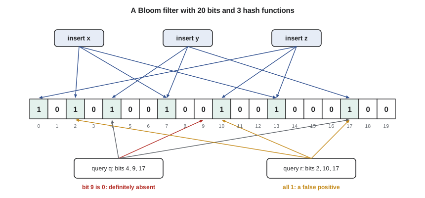
The server receives about 2.4 million records a night, and some arrive twice because a node retries an upload whose acknowledgment was lost. Checking each record against the full database index is slow. A Bloom filter, invented by Burton Bloom in 1970, answers the question 'have I seen this record before?' using a bit array of m bits and k independent hash functions. To insert a key, set the k bits it hashes to. To query, check those k bits: if any is 0 the key was definitely never inserted; if all are 1 it probably was.

A Bloom filter never gives false negatives but can give false positives, when other keys happen to have set all k bits. After inserting n keys, the false-positive rate is about (1 − e^(−kn/m))^k, minimized by choosing k ≈ (m/n) ln 2. With about 9.6 bits per key and seven hash functions, the rate is about 1 percent. Dana's ingest process keeps a Bloom filter of the last week's record identifiers, about 17 million keys, in about 20 MB of memory; only the roughly 1 percent of new records that the filter flags go to the slow exact check.

# A Bloom filter for duplicate upload detection, with measured false positives
import hashlib, math

class Bloom:
    def __init__(self, n, fp):
        self.m = math.ceil(-n * math.log(fp) / math.log(2) ** 2)
        self.k = max(1, round(self.m / n * math.log(2)))
        self.bits = bytearray((self.m + 7) // 8)
    def _idx(self, key):
        h = hashlib.sha256(key.encode()).digest()
        a, b = int.from_bytes(h[:8], 'big'), int.from_bytes(h[8:16], 'big')
        return [(a + i * b) % self.m for i in range(self.k)]
    def add(self, key):
        for i in self._idx(key):
            self.bits[i // 8] |= 1 << (i % 8)
    def __contains__(self, key):
        return all(self.bits[i // 8] >> (i % 8) & 1 for i in self._idx(key))

bf = Bloom(n=20000, fp=0.01)
for i in range(20000):
    bf.add(f"node{i % 400:03d}-rec{i}")
false_pos = sum(f"node{i % 400:03d}-rec{i}" in bf for i in range(20000, 40000))
print(f"bits per key: {bf.m / 20000:.1f}, hash functions: {bf.k}")
print(f"false positives on 20000 new keys: {false_pos} ({false_pos / 200:.2f} %)")
print("an inserted key is always found:", all(f"node{i % 400:03d}-rec{i}" in bf for i in range(0, 20000, 997)))

bits per key: 9.6, hash functions: 7
false positives on 20000 new keys: 192 (0.96 %)
an inserted key is always found: True

Reservoir sampling

The quality team audits a random sample of records each night by comparing them with video from a few cameras. They want exactly 100 records chosen uniformly at random from the night's stream, but the number of records is not known until the stream ends, and storing all of them first wastes memory. Reservoir sampling solves this in one pass with memory for only the sample. Keep the first 100 records. For the i-th record after that, with i counting from 1, generate a random integer r from 1 to i, and if r ≤ 100, replace the r-th record in the reservoir with the new one.

The proof is a short induction. Suppose after i − 1 records each has probability 100/(i − 1) of being in the reservoir. Record i enters with probability 100/i. An existing record survives step i unless the new record enters and replaces it, which happens with probability (100/i)·(1/100) = 1/i, so it survives with probability 100/(i − 1) · (1 − 1/i) = 100/i. Every record therefore ends with probability 100/N of being sampled, which is exactly uniform.

Concentration: how sure is 'probably'?

Expected values say what happens on average, but an engineer also needs to know how likely large deviations are. Markov's inequality gives a crude bound for any non-negative variable: the probability of exceeding a times the mean is at most 1/a. Chernoff bounds, for sums of independent indicator variables, give exponentially small tail probabilities: for example, a fair coin flipped 1,000 times shows more than 600 heads with probability less than about 2 × 10⁻⁹. Such bounds explain why randomized quicksort is not just fast on average but almost never slow, and why repeating a Monte Carlo test a few dozen times drives its error probability below the rate of hardware faults.