
CMP-301 · Lesson 11 of 12 · 19 min
NP-completeness: SAT, vertex cover, Hamiltonian cycles and the TSP
Lesson 10 defined NP-completeness and showed how reductions compare problems. A reduction proves hardness only if it starts from a problem already known to be hard, so the theory needs a first NP-complete problem, proved hard directly. That problem is Boolean satisfiability, and the proof that it is NP-complete, the Cook-Levin theorem, is one of the founding results of computer science. This lesson states the theorem and explains why it is true, then builds a chain of reductions from satisfiability to 3-SAT, independent set, vertex cover, Hamiltonian cycle, the traveling salesperson problem and subset sum. Along the way it shows the main gadget techniques used in hardness proofs.
The chain matters to Northway because two of its everyday problems sit on it. Gateway placement is a set cover problem, at least as hard as vertex cover. Planning the field crew's spring calibration route, visiting 38 sites and returning to the depot in the least driving time, is the traveling salesperson problem. Knowing both are NP-hard tells Dana where to stop looking for exact fast algorithms and start looking for good approximate ones.
Boolean satisfiability
A Boolean formula is built from variables that are true or false, using AND, OR and NOT. A formula in conjunctive normal form (CNF) is an AND of clauses, each clause an OR of literals, where a literal is a variable or its negation. The satisfiability problem, SAT, asks whether some assignment of truth values makes the formula true. The certificate is the assignment, and checking it means evaluating each clause, so SAT is in NP.
Satisfiability is a natural language for constraints. Maren's firmware build has dozens of optional features with dependencies and conflicts: compressed logging needs the newer flash driver, the newer flash driver conflicts with the legacy bootloader, the radar self-test needs either the newer driver or the debug UART. Asking whether some combination satisfies every rule, with a given set of features included, is a SAT question. Package managers in Linux distributions and in programming language ecosystems answer exactly this kind of question, and several of them use SAT solvers internally.
The Cook-Levin theorem
Stephen Cook in 1971, and independently Leonid Levin, proved that SAT is NP-complete. The idea of the proof is that any polynomial-time verifier can be described as a circuit, and a circuit can be described as a formula. Take any problem in NP, with a verifier that runs in time p(n) on inputs of length n. Its entire computation, step by step, fits in a table of p(n) rows and p(n) columns recording the machine's tape contents, head position and state at each time. Introduce Boolean variables for every cell of the table and every bit of the unknown certificate. Write clauses saying that the first row holds the input and the certificate, that each row follows from the previous one by the machine's rules, which are local and can be written cell by cell, and that the last row is in the accepting state.
The resulting formula has polynomially many variables and clauses, and it is satisfiable exactly when some certificate makes the verifier accept, that is, exactly when the original instance is a yes instance. So every problem in NP reduces to SAT. A year later, Richard Karp published reductions from SAT to 21 other problems, including vertex cover, Hamiltonian cycle and subset sum, establishing NP-completeness as a practical tool rather than a curiosity.
3-SAT
Reductions are easier to build from a problem with rigid structure. 3-SAT is SAT restricted to formulas in which every clause has exactly three literals. It is still NP-complete. A clause with more than three literals is split using new variables: (a ∨ b ∨ c ∨ d) becomes (a ∨ b ∨ y) ∧ (¬y ∨ c ∨ d), where y is new. If the original clause is true, some literal is true and y can be chosen to satisfy both new clauses; if both new clauses are true, then whatever y is, one of a, b, c, d is true. Short clauses are padded with copies of literals. The transformation is linear in the size of the formula.
By contrast, 2-SAT, where every clause has two literals, is in P: it reduces to finding strongly connected components in an implication graph, linear time. The jump from two literals to three is the jump from easy to hard, a pattern that recurs throughout complexity theory, as with 2-coloring (easy, it is bipartiteness) and 3-coloring (NP-complete).
3-SAT to independent set
The reduction from 3-SAT to independent set is the standard first example of a gadget proof. Given a 3-SAT formula with m clauses, build a graph with a triangle for each clause, one vertex per literal in the clause. Then add an edge between every pair of vertices that are complementary literals, x in one clause and ¬x in another. Ask whether the graph has an independent set of size m.
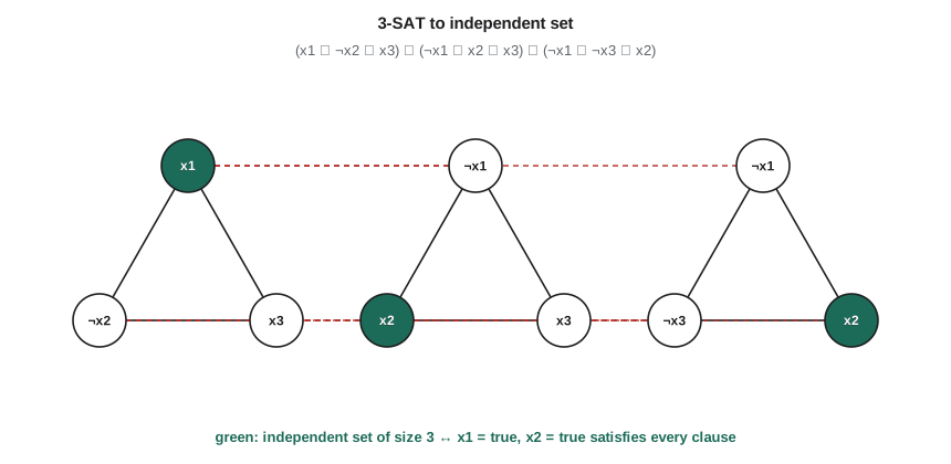
If the formula is satisfiable, take a satisfying assignment and pick one true literal from each clause; those m vertices are independent, because each triangle contributes one and no two chosen literals are complementary, since they are all true. Conversely, an independent set of size m must take exactly one vertex from each triangle, because the triangle's vertices are pairwise adjacent, and it never takes both x and ¬x. Setting each chosen literal true, and any unmentioned variable arbitrarily, satisfies every clause. The graph has 3m vertices and is built in polynomial time, so independent set is NP-complete, and by lesson 10's complement argument, so are vertex cover and clique.
Hamiltonian cycle and the traveling salesperson problem
A Hamiltonian cycle visits every vertex of a graph exactly once and returns to the start. Deciding whether one exists is NP-complete, by a reduction from 3-SAT that builds a gadget for each variable, a long chain that can be traversed left-to-right (true) or right-to-left (false), and a gadget for each clause, a vertex that the cycle can detour to only from a chain traversed in a direction that makes one of the clause's literals true. The details are intricate but the principle is the same as before: gadgets whose only possible behaviors correspond to truth values, wired so that global consistency means a satisfying assignment.
The traveling salesperson problem (TSP) asks, given distances between n cities and a budget B, whether some tour visiting every city once has total length at most B. Hamiltonian cycle reduces to it immediately. Given a graph, make each edge distance 1 and each non-edge distance 2, and set B = n. A tour of length n uses only distance-1 steps, which means only edges of the original graph, so it is a Hamiltonian cycle; conversely a Hamiltonian cycle gives a tour of length n. TSP is in NP, since a tour is checked by adding its length, so TSP is NP-complete.
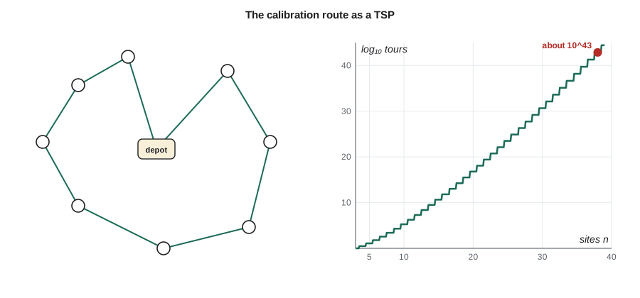
The field crew's route has 38 sites plus the depot. The number of distinct tours is (n − 1)!/2, about 10⁴⁴ for 39 locations, so checking them all is impossible. Dynamic programming over subsets, the Held-Karp algorithm from 1962, solves TSP exactly in O(n²·2ⁿ) time, which is far better than n! but still exponential: it handles about 25 cities on a laptop and is useless at 39. Lesson 12 shows how practical solvers get within a fraction of a percent of optimal on such instances in seconds.
# Held-Karp dynamic programming for an exact small TSP (travel times in minutes)
from itertools import combinations

names = ['Depot', 'Bath Rd', 'Front St', 'Hwy 15', 'Lake Rd', 'Mill Rd', 'Station Rd']
D = [[0, 12, 9, 22, 17, 25, 14],
     [12, 0, 7, 18, 20, 16, 11],
     [9, 7, 0, 15, 13, 21, 6],
     [22, 18, 15, 0, 10, 8, 19],
     [17, 20, 13, 10, 0, 14, 12],
     [25, 16, 21, 8, 14, 0, 23],
     [14, 11, 6, 19, 12, 23, 0]]
n = len(D)
best = {(1 << j, j): (D[0][j], 0) for j in range(1, n)}
for size in range(2, n):
    for subset in combinations(range(1, n), size):
        mask = sum(1 << j for j in subset)
        for j in subset:
            prev = mask & ~(1 << j)
            best[(mask, j)] = min((best[(prev, k)][0] + D[k][j], k) for k in subset if k != j)
full = (1 << n) - 2
length, last = min((best[(full, j)][0] + D[j][0], j) for j in range(1, n))
tour, mask, j = [], full, last
while j:
    tour.append(names[j]); mask, j = mask & ~(1 << j), best[(mask, j)][1]
print("optimal tour: Depot ->", " -> ".join(reversed(tour)), "-> Depot")
print("length:", length, "minutes; table entries:", len(best))optimal tour: Depot -> Front St -> Station Rd -> Lake Rd -> Hwy 15 -> Mill Rd -> Bath Rd -> Depot length: 73 minutes; table entries: 192
Subset sum and knapsack
Subset sum asks whether some subset of given integers adds up exactly to a target T. It is NP-complete, by a reduction from 3-SAT that writes numbers in base 10 with one digit position per variable and one per clause, arranging the digits so that choosing numbers corresponds to choosing truth values and each clause digit can only reach its target if some literal in the clause is true. Subset sum reduces to the decision version of 0/1 knapsack by setting each item's size and value equal to its number and asking for value at least T within capacity T, so knapsack is NP-complete too.
That seems to contradict lesson 4, which solved knapsack by dynamic programming. It does not. The dynamic program runs in Θ(nW) time, polynomial in the numeric value W but exponential in its bit length. The reduction from 3-SAT produces numbers with as many digits as there are variables and clauses, so W is exponentially large in the formula size, and the dynamic program is exponential on those instances. Problems that are NP-complete but have pseudo-polynomial algorithms are called weakly NP-complete; those that stay hard even when the numbers are small, such as bin packing and TSP, are strongly NP-complete.
A gallery of NP-complete problems
| Problem | Where it appears | Reduced from |
|---|---|---|
| SAT, 3-SAT | Configuration, verification, planning | Every NP problem (Cook-Levin) |
| Independent set, clique, vertex cover | Placement, conflict resolution | 3-SAT |
| Set cover | Sensor and gateway placement | Vertex cover |
| Hamiltonian cycle, TSP | Routing, drilling, delivery | 3-SAT |
| Graph coloring (k ≥ 3) | Frequency assignment, register allocation, timetabling | 3-SAT |
| Subset sum, knapsack, partition | Budgeting, load balancing | 3-SAT |
| Bin packing | Packing uploads into time slots | Partition |
| Integer linear programming | General optimization | SAT |
| Job shop scheduling | Manufacturing, server jobs | Partition, 3-SAT |
Recognizing these problems in disguise is the practical skill. Assigning radio channels to gateways so that neighbors never share a channel is graph coloring. Packing a night's upload batches into fixed-size time slots on the cellular link is bin packing. Choosing which counters to visit with a limited crew budget to maximize data recovered is a knapsack with routing on top. When a new problem looks like one of these, a quick reduction attempt either reveals a special structure that makes it easy, as with trees in lesson 5 or bipartite graphs in lesson 6, or confirms that it is hard.
Worked problem
Splitting a long clause for 3-SAT
Convert the clause (a ∨ ¬b ∨ c ∨ d ∨ ¬e) into an equivalent set of 3-literal clauses for satisfiability.
Show solution
- Introduce new variables y₁ and y₂.
- First clause: (a ∨ ¬b ∨ y₁).
- Middle clause: (¬y₁ ∨ c ∨ y₂).
- Last clause: (¬y₂ ∨ d ∨ ¬e).
- If some original literal is true, set the y variables so that every new clause containing it is satisfied and the others are satisfied by a y; if all original literals are false, the chain forces y₁ true, then y₂ true, and the last clause fails.
Answer: A clause with k literals becomes k − 2 clauses with k − 3 new variables, so the conversion is linear in the formula size.
Common mistakes
MistakeProving NP-hardness by showing the problem's brute force is exponential.
InsteadBrute force says nothing about hardness. Reduce a known NP-complete problem to the new one and prove both directions.
MistakeCalling knapsack polynomial because of the Θ(nW) dynamic program.
InsteadThat is pseudo-polynomial. Knapsack is weakly NP-complete: hard when the numbers have many digits.
MistakeAssuming 2-SAT is hard because SAT is.
Instead2-SAT is solvable in linear time with an implication graph. Restricted versions of hard problems are often easy.
MistakeReducing in the wrong direction when building a hardness gadget.
InsteadInstances of the known hard problem must be transformed into instances of the new problem, not the other way around.
Summary and key terms
- The Cook-Levin theorem shows SAT is NP-complete by encoding any polynomial-time verification as a formula.
- 3-SAT is NP-complete; long clauses split with new variables, while 2-SAT is solvable in linear time.
- The triangle gadget reduces 3-SAT to independent set, making vertex cover and clique NP-complete.
- Hamiltonian cycle is NP-complete, and setting edge weights 1 and non-edges 2 reduces it to TSP.
- Subset sum and knapsack are weakly NP-complete: hard with large numbers, pseudo-polynomial with small ones.
- Recognizing NP-complete problems in disguise, such as coloring, bin packing and set cover, guides engineering choices.
- Satisfiability (SAT)
- Deciding whether some truth assignment makes a Boolean formula true.
- Conjunctive normal form
- An AND of clauses, each an OR of literals.
- Cook-Levin theorem
- The result that SAT is NP-complete, proved by encoding verifier computations as formulas.
- Gadget
- A small structure in a reduction whose possible behaviors mirror choices in the source problem.
- Hamiltonian cycle
- A cycle that visits every vertex of a graph exactly once.
- Traveling salesperson problem
- Finding a shortest tour that visits every city once and returns to the start.
- Weakly NP-complete
- NP-complete but solvable in pseudo-polynomial time, as with knapsack and subset sum.
Practice problems
Work each problem on paper first, then reveal the answer to check.
Is (x ∨ y) ∧ (¬x ∨ y) ∧ (¬y ∨ z) ∧ (¬z ∨ ¬y) satisfiable?
Show answer
No. The first two clauses force y true; then the third forces z true and the fourth requires z false.
How many vertices does the independent-set graph have for a 3-SAT formula with 40 clauses, and what size of independent set is asked for?
Show answer
120 vertices (three per clause) and an independent set of size 40.
How many distinct tours does a TSP with 10 cities have?
Show answer
(10 − 1)!/2 = 181,440.
Why is TSP in NP but Held-Karp not a polynomial algorithm?
Show answer
A tour is checked in linear time, but Held-Karp's table has n·2ⁿ entries, exponential in n.
Lesson quiz · 5 questions
Score 60% or more to complete this lesson.
Create a free account to save your progress, take quizzes and earn a certificate.