Dynamic programming I: memoization, knapsack and subsequences

Dynamic programming solves problems whose subproblems overlap. Where divide and conquer splits a problem into independent pieces, dynamic programming recognizes that the same smaller problems come up again and again, solves each one once, stores its answer in a table and looks it up whenever it is needed. The idea turns many exponential searches into polynomial algorithms. It is also the paradigm students find hardest at first, because the clever part is not the code, which is usually a few nested loops, but the choice of subproblems. This lesson builds the method on three problems Northway actually meets: weighted interval scheduling, the 0/1 knapsack and the longest common subsequence.

The name is historical. Richard Bellman coined it in the 1950s, choosing 'programming' in its older sense of planning, as in a television programming schedule, and 'dynamic' because the plans unfolded over time. Nothing about it involves writing programs dynamically.

Overlapping subproblems: a first example

Lesson 2 showed that greedy fails for change-making with coins of 1, 3 and 4. A natural fix is to try every coin first and recurse on what remains: the fewest coins for amount a is one more than the best of the fewest coins for a − 1, a − 3 and a − 4. The recursion is correct but slow, because the same amounts are recomputed many times. Computing amount 30 calls amount 26 by several different routes, each of which recomputes everything below it. The number of calls grows exponentially with the amount.

Memoization fixes this by storing each answer the first time it is computed and returning the stored answer on later calls. With memoization each amount from 0 to a is computed once, using constant work per coin, so the total is Θ(a·k) for k coin types. The second way to organize the same computation is tabulation, also called the bottom-up method: fill a table in an order that guarantees each entry's dependencies are already filled. Both give the same answers and the same asymptotic cost. Memoization is often easier to write; tabulation avoids recursion depth limits and usually runs faster.

# Fewest coins: plain recursion vs memoization vs a bottom-up table
from functools import lru_cache
coins = (1, 3, 4)
calls = [0]

def plain(a):
    calls[0] += 1
    if a == 0:
        return 0
    return 1 + min(plain(a - c) for c in coins if c <= a)

@lru_cache(maxsize=None)
def memo(a):
    if a == 0:
        return 0
    return 1 + min(memo(a - c) for c in coins if c <= a)

def table(amount):
    best = [0] + [float('inf')] * amount
    for a in range(1, amount + 1):
        best[a] = 1 + min(best[a - c] for c in coins if c <= a)
    return best[amount]

for amt in (6, 15, 24):
    calls[0] = 0
    p = plain(amt)
    print(f"amount {amt:2d}: plain={p} ({calls[0]:7d} calls)  memo={memo(amt)}  table={table(amt)}")

amount  6: plain=2 (     24 calls)  memo=2  table=2
amount 15: plain=4 (   1869 calls)  memo=4  table=4
amount 24: plain=6 ( 142129 calls)  memo=6  table=6

The four steps of dynamic programming

Every dynamic program in this course is designed in the same four steps. First, define the subproblems precisely in words, including what their parameters mean; this is the step that requires insight. Second, write the recurrence that expresses each subproblem in terms of smaller ones, together with base cases. Third, choose an evaluation order in which every subproblem's dependencies come first, and decide how much of the table must be kept. Fourth, recover the actual solution, not just its value, by recording which choice achieved each optimum and tracing back from the final entry.

Correctness rests on the principle of optimality: an optimal solution to the whole problem contains optimal solutions to its subproblems. When this holds, the recurrence is correct by induction on subproblem size. Running time is the number of subproblems times the work per subproblem, plus the cost of the traceback.

Weighted interval scheduling

Dana revisits the upload windows from lesson 2 with a twist. The carrier now offers windows of different value: an upload in some windows saves more money than in others, because of time-of-day pricing and the size of each node's batch. Each request j has a start s_j, finish f_j and value v_j, and the goal is a set of non-overlapping requests with the largest total value. Earliest finish time no longer works, because one valuable long window can be worth more than two short cheap ones.

Sort the requests by finish time and number them 1 to n. Let p(j) be the largest index i < j whose request finishes no later than j starts, or 0 if there is none. Define OPT(j) as the best total value using only requests 1 to j. Either request j is in the optimal solution for 1 to j, in which case it contributes v_j and the rest comes from requests compatible with it, 1 to p(j); or it is not, in which case the answer is OPT(j − 1).

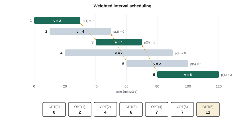
There are n subproblems and each takes constant time once p(j) is known. Computing all p(j) values takes O(n log n) by binary search over the sorted finish times, so the whole algorithm runs in O(n log n). Tracing back from OPT(n), taking request j whenever v_j + OPT(p(j)) ≥ OPT(j − 1), recovers the chosen windows.

# Weighted interval scheduling with traceback
import bisect

reqs = [  # (start, finish, value) in minutes after 01:00
    (0, 30, 2), (10, 50, 4), (40, 70, 4), (20, 90, 7), (60, 100, 2), (80, 120, 5)]
reqs.sort(key=lambda r: r[1])
finishes = [r[1] for r in reqs]
n = len(reqs)
p = [bisect.bisect_right(finishes, reqs[j][0]) for j in range(n)]   # count of requests ending by start

opt = [0] * (n + 1)
for j in range(1, n + 1):
    s, f, v = reqs[j - 1]
    opt[j] = max(v + opt[p[j - 1]], opt[j - 1])

chosen, j = [], n
while j > 0:
    s, f, v = reqs[j - 1]
    if v + opt[p[j - 1]] >= opt[j - 1]:
        chosen.append((s, f, v)); j = p[j - 1]
    else:
        j -= 1
print("OPT table:", opt)
print("chosen windows:", sorted(chosen), "total value", opt[n])

OPT table: [0, 2, 4, 6, 7, 7, 11]
chosen windows: [(0, 30, 2), (40, 70, 4), (80, 120, 5)] total value 11

The 0/1 knapsack problem

Maren's firmware question from lesson 2 is next. The NS-4's flash has 64 KB free for optional features. Each candidate feature has a size in kilobytes and a value, a score the product team assigned from customer requests. Features cannot be split. Choose the subset with the largest total value whose sizes add up to at most 64 KB. This is the 0/1 knapsack problem.

The single index used for interval scheduling is not enough here, because whether item j fits depends on how much capacity earlier choices used. The fix, and a pattern worth remembering, is to add a parameter: let OPT(j, w) be the best value using items 1 to j with capacity w. Either item j is left out, giving OPT(j − 1, w), or, if it fits, it is taken, giving v_j + OPT(j − 1, w − w_j).

The table has (n + 1)(W + 1) entries for n items and capacity W, each filled in constant time, so the algorithm runs in Θ(nW) time. Because each row depends only on the row above, the memory can be reduced to two rows, or even one row filled from high capacity to low, Θ(W) in total, at the cost of a more involved traceback.

# 0/1 knapsack by dynamic programming, with traceback, compared with greedy
def knapsack(items, W):
    n = len(items)
    opt = [[0] * (W + 1) for _ in range(n + 1)]
    for j in range(1, n + 1):
        name, w, v = items[j - 1]
        for cap in range(W + 1):
            opt[j][cap] = opt[j - 1][cap]
            if w <= cap and v + opt[j - 1][cap - w] > opt[j][cap]:
                opt[j][cap] = v + opt[j - 1][cap - w]
    chosen, cap = [], W
    for j in range(n, 0, -1):
        if opt[j][cap] != opt[j - 1][cap]:
            name, w, v = items[j - 1]; chosen.append(name); cap -= w
    return opt[n][W], sorted(chosen)

def greedy(items, W):
    total, used, chosen = 0, 0, []
    for name, w, v in sorted(items, key=lambda it: -it[2] / it[1]):
        if used + w <= W:
            used += w; total += v; chosen.append(name)
    return total, sorted(chosen)

features = [('selftest', 12, 30), ('logging', 20, 45), ('reconfig', 28, 60),
            ('classify', 34, 70), ('forecast', 16, 25)]
print("64 KB  dp:", knapsack(features, 64), " greedy:", greedy(features, 64))

tight = [('bootloader_v2', 40, 82), ('diagnostics', 30, 60), ('ota_delta', 30, 60)]
print("60 KB  dp:", knapsack(tight, 60), " greedy:", greedy(tight, 60))

64 KB  dp: (135, ['logging', 'reconfig', 'selftest'])  greedy: (135, ['logging', 'reconfig', 'selftest'])
60 KB  dp: (120, ['diagnostics', 'ota_delta'])  greedy: (82, ['bootloader_v2'])

The second instance shows the failure. The bootloader update has the best ratio, 2.05 per kilobyte, so greedy takes it and then cannot fit either 30 KB feature, scoring 82. The dynamic program takes the two 30 KB features for 120. On the NS-4's real list of 23 candidate features, the difference between greedy and optimal was worth about 15 percent of the total value, enough that Maren adopted the dynamic program for every release plan.

Pseudo-polynomial time

The knapsack algorithm's Θ(nW) running time looks polynomial, but W is a number, and as lesson 1 noted, its size in the input is the number of bits, log₂ W. If capacities were measured in bytes rather than kilobytes, W would be 65,536 instead of 64 and the table a thousand times larger, though the problem is the same. An algorithm polynomial in the numeric values but not in their bit lengths is called pseudo-polynomial. Lesson 11 shows that knapsack is NP-hard, so no truly polynomial algorithm is expected, and lesson 12 shows how scaling the values gives a fast approximation with a guaranteed error.

Longest common subsequence

A third family of dynamic programs works on two sequences. Northway's nodes store their configuration as an ordered list of settings, and when a node misbehaves the support team compares its configuration with the standard one. A subsequence keeps some elements in their original order, possibly with gaps; the longest common subsequence (LCS) of two sequences is the longest sequence that is a subsequence of both. The settings not in the LCS are exactly what a diff tool reports as additions and deletions.

For sequences x of length m and y of length n, let L(i, j) be the length of the LCS of the first i elements of x and the first j elements of y. If the last elements match, they can end a common subsequence; otherwise one of them must be left out.

The table has (m + 1)(n + 1) entries, each filled in constant time, so the algorithm runs in Θ(mn) time and space. Diff tools compare files line by line in exactly this way, though practical ones use refinements that run much faster when the files are mostly the same. Lesson 5 extends the idea to edit distance, which assigns costs to insertions, deletions and substitutions, and to sequence alignment.

# Longest common subsequence of two configuration lists, with traceback
def lcs(x, y):
    m, n = len(x), len(y)
    L = [[0] * (n + 1) for _ in range(m + 1)]
    for i in range(1, m + 1):
        for j in range(1, n + 1):
            if x[i - 1] == y[j - 1]:
                L[i][j] = L[i - 1][j - 1] + 1
            else:
                L[i][j] = max(L[i - 1][j], L[i][j - 1])
    out, i, j = [], m, n
    while i and j:
        if x[i - 1] == y[j - 1]:
            out.append(x[i - 1]); i -= 1; j -= 1
        elif L[i - 1][j] >= L[i][j - 1]:
            i -= 1
        else:
            j -= 1
    return out[::-1]

standard = ['radar=on', 'gain=12', 'bins=15min', 'classes=8', 'upload=02:00', 'gps=on']
node_217 = ['radar=on', 'gain=18', 'bins=15min', 'upload=02:00', 'gps=off', 'debug=on']
common = lcs(standard, node_217)
print("common:", common)
print("removed:", [s for s in standard if s not in common])
print("added:  ", [s for s in node_217 if s not in common])

common: ['radar=on', 'bins=15min', 'upload=02:00']
removed: ['gain=12', 'classes=8', 'gps=on']
added:   ['gain=18', 'gps=off', 'debug=on']