
CMP-301 · Lesson 1 of 12 · 22 min
Algorithm design: paradigms, correctness and cost
A data structure course teaches you how to store information so that the operations you need are cheap. An algorithm design course asks a harder question: given a problem nobody has handed you a recipe for, how do you invent a method that is correct, prove that it is correct, and know how much time and memory it will use before you write a line of production code? This course answers that question with a small number of design paradigms that recur across computer engineering: greedy choice, divide and conquer, dynamic programming, network flow, randomization and amortization. It then turns to the uncomfortable truth that some problems have no known efficient algorithm at all, and to what engineers do about them.
The course continues at Northway Sensing in Ann Arbor, Michigan, the company that builds the NS-4 solar-powered roadside traffic counter. Jonah Abara, now a junior on a co-op term, has moved from the firmware bench to the server team, which collects counts from about 400 deployed nodes, stores them, and produces the reports that city and county traffic engineers use. His supervisor is Dana Okoye, the back-end lead, and Maren Holt, the firmware lead from CMP-200, still appears whenever a decision touches the devices themselves.
Prerequisites matter here. CMP-200 introduced Big-O notation, arrays, lists, trees, heaps and hash tables, and CMP-250 covered proof by induction, sets, counting and graphs. CMPUT-204 Algorithms I, which many students take alongside this course, treats sorting lower bounds, shortest paths and minimum spanning trees in detail. This course refers to those results rather than re-deriving them and spends its time on design techniques and on the limits of computation.
What a problem and an algorithm are
A computational problem is a precise relationship between inputs and acceptable outputs. 'Sort these upload records by timestamp' is a problem: the input is any finite list of records and the acceptable output is the same records in non-decreasing timestamp order. An instance is one particular input. An algorithm is a finite, unambiguous procedure that, for every instance, halts and produces an acceptable output. The word every carries the weight. A method that works on the test data but fails on an input nobody tried is not an algorithm for the problem; it is a bug waiting for the right input.
Engineers often meet problems first as vague requests. Dana's first request to Jonah is typical: 'The cellular bill went up again. Can you make the nodes upload more cheaply?' Before any algorithm can be designed, that request has to become a problem with inputs, outputs and an objective. After a morning of questions, Jonah writes it down: each node has a batch of data ready at a known time, each batch must reach the server before a known deadline, the carrier charges more during busy hours, and the server can accept only a limited number of simultaneous uploads. Choose an upload time for each batch that meets every deadline and minimizes cost. That formulation, refined over the term, is the capstone problem of lesson 12.
The design paradigms
Most efficient algorithms are built from a handful of ideas. Recognizing which idea fits a problem is the main skill this course develops, and the table below previews them. The paradigms are not mutually exclusive: many practical algorithms combine several, such as a divide-and-conquer algorithm whose subproblems are solved greedily.
| Paradigm | Core idea | Typical examples | Lesson |
|---|---|---|---|
| Greedy | Make the locally best choice and never undo it | Interval scheduling, Huffman codes, Dijkstra | 2 |
| Divide and conquer | Split into independent subproblems, solve recursively, combine | Merge sort, Karatsuba, closest pair | 3 |
| Dynamic programming | Solve overlapping subproblems once and reuse the answers | Knapsack, edit distance, Bellman-Ford | 4, 5, 7 |
| Network flow | Model the problem as moving flow through a capacitated graph | Max flow, bipartite matching | 6 |
| Randomization | Use random choices to get good expected behavior | Quickselect, hashing, sampling | 8 |
| Amortization | Pay for rare expensive steps with many cheap ones | Dynamic arrays, union-find | 9 |
| Reduction | Solve one problem by transforming it into another | Matching via flow, NP-hardness proofs | 6, 10, 11 |
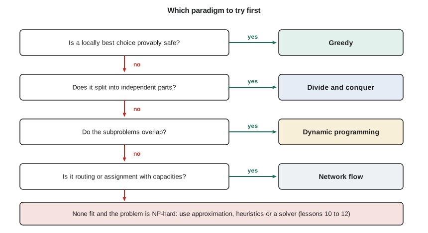
Correctness: why an algorithm works
An algorithm is correct if it halts on every instance with an acceptable output. Testing can show that an algorithm is wrong, by finding an instance where it fails, but it cannot show that it is right, because there are infinitely many instances. Proof is the only way to be sure, and the habit of proving correctness, even informally, catches design errors that no test suite would. Three proof techniques do most of the work in this course.
The first is the loop invariant, a statement about the program's variables that is true before the loop starts, stays true after each iteration, and, together with the loop's exit condition, implies the result. You met invariants in CMP-200 when reasoning about binary search. The second is induction on the input size, which suits recursive algorithms: assume the algorithm is correct on all smaller inputs and show it is correct on the current one. The third is the exchange argument, which suits greedy algorithms: take any optimal solution, show it can be transformed step by step into the greedy solution without getting worse, and conclude that the greedy solution is also optimal. Lesson 2 uses exchange arguments throughout.
Worked problem
A loop invariant for the maximum gap
Dana wants a quick check of data quality: given the sorted upload timestamps from one node over a day, find the longest gap between consecutive uploads. Jonah writes a single loop that keeps the largest difference seen so far. State an invariant and use it to argue that the loop is correct.
Show solution
- Let the timestamps be t[0] ≤ t[1] ≤ … ≤ t[n−1], and let best start at 0 before the loop over i = 1, …, n − 1.
- Invariant: at the start of iteration i, best equals the largest of t[k] − t[k−1] for 1 ≤ k < i, or 0 if there are none.
- Initialization: at i = 1 the set of earlier gaps is empty and best = 0, so the invariant holds.
- Maintenance: the iteration sets best to the larger of best and t[i] − t[i−1], so afterwards best is the largest gap with k < i + 1.
- Termination: the loop ends with i = n, so best is the largest of all gaps t[k] − t[k−1] for 1 ≤ k < n.
Answer: The invariant proves the loop correct for every input, including the edge cases a test suite might miss: one timestamp gives best = 0 and two identical timestamps give a gap of 0. Writing the invariant took less time than writing the tests.
Cost: measuring running time
The second question about any algorithm is how its cost grows with the size of the input. As in CMP-200, we count basic operations rather than seconds, because seconds depend on the processor, the compiler and the cache, while the growth rate depends only on the algorithm. We usually report the worst case, the largest cost over all inputs of size n, because a guarantee is more useful than a hope. Sometimes the average case, over a stated distribution of inputs, or the amortized cost, averaged over a sequence of operations, is the more honest measure; lessons 8 and 9 develop those.
Big-O gives an upper bound, Big-Omega a lower bound and Big-Theta both at once. A statement such as 'merge sort runs in Θ(n log n) time' means that its worst case grows exactly as fast as n log n, up to constant factors. Constant factors matter in practice, and later lessons point out where they do, but the growth rate decides which algorithms remain usable as data grows. Northway's database already holds about 2.1 billion count records, and an algorithm that is quadratic in the number of records will never finish on it, however fast the server.
| Growth rate | n = 1,000 | n = 1,000,000 | Typical source |
|---|---|---|---|
| log n | 10 | 20 | Binary search, balanced trees |
| n | 1,000 | 1,000,000 | A single pass over the data |
| n log n | 10,000 | 20,000,000 | Sorting, divide and conquer |
| n² | 1,000,000 | 10¹² | All pairs, simple dynamic programs |
| n³ | 10⁹ | 10¹⁸ | Floyd-Warshall, matrix multiplication |
| 2ⁿ | about 10³⁰¹ | unthinkable | Trying every subset |
Polynomial time as the working definition of efficient
Throughout this course an algorithm is called efficient if its worst-case running time is bounded by a polynomial in the input size, such as n, n log n or n³. The definition is crude: an n¹⁰⁰ algorithm is useless and a 1.0001ⁿ algorithm may be fine for the inputs anyone meets. It has survived for decades because it matches practice surprisingly well. Problems with polynomial algorithms usually have ones with small exponents, and exponential algorithms usually blow up at modest sizes. The distinction between polynomial and exponential time is also the foundation of the theory of NP-completeness in lessons 10 and 11.
Input size needs care. For a list of n records the size is n. For a number N given in binary, the size is the number of bits, about log₂ N. An algorithm that loops N times is therefore exponential in the input size even though it looks linear in N. This distinction, between running time polynomial in the numeric value and polynomial in the number of bits, explains why the dynamic program for knapsack in lesson 4 is called pseudo-polynomial.
Recurrences
Recursive algorithms have running times described by recurrences, equations that express the cost on an input of size n in terms of the cost on smaller inputs. Merge sort splits n items into two halves, sorts each recursively and merges in linear time, so its cost satisfies T(n) = 2T(n/2) + cn. Solving recurrences is a core skill of algorithm analysis. Lesson 3 introduces the master theorem, which solves the most common family at a glance, and the recursion tree method that explains it.
Lower bounds and optimality
Knowing that an algorithm runs in O(n log n) time is half the story. The other half is knowing whether any algorithm could do better. A lower bound is a proof that every algorithm for a problem, in some model of computation, needs at least a certain amount of work. CMPUT-204 proves that any comparison-based sorting algorithm needs Ω(n log n) comparisons in the worst case, so merge sort and heapsort are optimal in that model. When an algorithm's running time matches the lower bound, the design work is done; when it does not, there may be room to improve.
Some lower bounds are easy. Any algorithm that must look at every input item takes at least Ω(n) time, which is why finding the largest gap in a list cannot be done faster than one pass. Others are among the hardest open questions in mathematics. Nobody has proved that the problems in lesson 11 need exponential time, even though decades of effort have failed to find polynomial algorithms for them.
Experiments complement analysis
Analysis predicts growth rates, and experiments check the prediction and measure constants. A useful experiment counts operations, which is deterministic and portable, rather than timing them, which varies from run to run. The code below counts the comparisons made by insertion sort and merge sort on the same deterministic pseudo-random input and shows the quadratic and n log n growth predicted by analysis. Doubling n roughly quadruples insertion sort's comparisons and roughly doubles merge sort's.
# Count comparisons to check growth rates experimentally (deterministic input)
def lcg(seed):
    while True:
        seed = (1103515245 * seed + 12345) % 2**31
        yield seed

def insertion(a):
    a = a[:]; comps = 0
    for i in range(1, len(a)):
        x, j = a[i], i - 1
        while j >= 0:
            comps += 1
            if a[j] <= x:
                break
            a[j + 1] = a[j]; j -= 1
        a[j + 1] = x
    return comps

def merge_count(a):
    if len(a) <= 1:
        return a, 0
    m = len(a) // 2
    left, c1 = merge_count(a[:m]); right, c2 = merge_count(a[m:])
    out, i, j, c = [], 0, 0, c1 + c2
    while i < len(left) and j < len(right):
        c += 1
        if left[i] <= right[j]:
            out.append(left[i]); i += 1
        else:
            out.append(right[j]); j += 1
    return out + left[i:] + right[j:], c

g = lcg(42)
print("     n   insertion      merge")
for n in (500, 1000, 2000, 4000):
    data = [next(g) % 100000 for _ in range(n)]
print(f"{n:6d} {insertion(data):11d} {merge_count(data)[1]:10d}")n insertion merge 500 63095 3851 1000 249263 8699 2000 993604 19382 4000 4019312 42796
The numbers make the abstract table concrete. At 4,000 records insertion sort already needs about four million comparisons while merge sort needs about 43,000, and the ratio keeps widening. Jonah's sorting of a single node's day of data, about 300 records, would never show the difference; sorting the whole archive would show nothing else.
The design process
Designing an algorithm in practice is iterative. Formulate the problem precisely, with inputs, outputs and objective. Work small examples by hand, because patterns that suggest a paradigm usually appear in the first few. Try the simplest correct method, often brute force, and analyze its cost; it is the baseline every clever idea must beat, and it is the test oracle for the clever version. Look for structure: a safe greedy choice, a split into independent parts, overlapping subproblems, a flow network. Prove the improved algorithm correct and analyze it. Then implement, test against the brute force on many small inputs, and measure on realistic data.
The brute-force baseline deserves emphasis. For the upload problem, trying every assignment of upload slots to 400 nodes is hopeless, but trying every assignment for five nodes and six slots is instant. Comparing a clever algorithm with brute force on thousands of random small instances catches most bugs before any real data is touched, and it is the single most useful testing habit in algorithm work.
Common mistakes
MistakeTreating an algorithm that passes the test suite as proven correct.
InsteadTests can only show failure. State an invariant, an induction hypothesis or an exchange argument, and test against brute force on many small instances.
MistakeMeasuring input size by the numeric value of a number rather than by its length in bits.
InsteadThe size of a number N is about log₂ N bits, so a loop that runs N times is exponential in the input size.
MistakeComparing algorithms by timing one run on one machine.
InsteadCount operations or analyze growth rates. Timings depend on hardware, caching and load, and a single run hides how cost grows.
MistakeDesigning before formulating: starting to code from a vague request.
InsteadWrite down the inputs, the acceptable outputs and the objective first. Many hard problems turn out to be easy, or easy ones hard, once stated precisely.
Summary and key terms
- A problem relates inputs to acceptable outputs; an algorithm halts on every instance with an acceptable output.
- The main paradigms are greedy, divide and conquer, dynamic programming, network flow, randomization, amortization and reduction.
- Correctness is proved with loop invariants, induction or exchange arguments; testing can only reveal errors.
- Running time is measured by growth rate in the worst case, with average-case and amortized measures where they are more informative.
- Polynomial time is the working definition of efficient; input size for numbers is their length in bits.
- Lower bounds show when an algorithm is optimal; a brute-force baseline is the reference for testing clever algorithms.
- Instance
- One particular input to a computational problem.
- Loop invariant
- A statement that holds before a loop and after every iteration, used to prove the loop correct.
- Exchange argument
- A proof that a greedy solution is optimal by transforming any optimal solution into it without loss.
- Worst-case running time
- The largest cost of an algorithm over all inputs of a given size.
- Polynomial time
- Running time bounded by n raised to a fixed power, where n is the input size.
- Lower bound
- A proof that every algorithm for a problem needs at least a certain amount of work.
- Pseudo-polynomial
- Running time polynomial in the numeric values in the input but exponential in their length in bits.
Practice problems
Work each problem on paper first, then reveal the answer to check.
Write an invariant for a loop that computes the sum of a list.
Show answer
At the start of iteration i, total equals the sum of a[0] through a[i−1]. It holds initially (empty sum is 0), each iteration adds a[i], and at exit total is the sum of all n items.
An algorithm loops N times on input N given in binary. Is it polynomial?
Show answer
No. The input has about log₂ N bits, so N = 2^(bits), and the running time is exponential in the input size.
Rank n², n log n, 2ⁿ and n³ by growth.
Show answer
n log n, then n², then n³, then 2ⁿ.
Why test a fast algorithm against brute force on small inputs?
Show answer
Brute force is easy to get right, so disagreements reveal bugs in the fast algorithm across thousands of cases no person would think to write.
Lesson quiz · 5 questions
Score 60% or more to complete this lesson.
Create a free account to save your progress, take quizzes and earn a certificate.