
CMP-200 · Lesson 2 of 12 · 20 min
Algorithm analysis and Big-O notation
Lesson 1 counted the comparisons a linear search makes and found that the count grows in proportion to the number of records. This lesson turns that observation into a tool. Asymptotic analysis describes how the cost of an algorithm grows as the input gets large, ignoring constant factors and small terms that depend on the machine. Its notation, Big-O and its relatives, is the shared language engineers use in design reviews, documentation and job interviews: a hash table lookup is O(1) on average, binary search is O(log n), sorting by comparisons is O(n log n) at best. Knowing what these statements mean, and what they do not mean, lets you predict whether a design will still work when the data grows by a factor of a thousand.
Jonah's first real task shows why this matters. The Northway server checks every new batch of vehicle records for duplicates, because a node that loses its cellular connection mid-upload resends the whole batch. The original check, written in a hurry, compared every new record with every record already stored for that node that day. It worked perfectly in testing with a few hundred records. In production, a busy highway node produces about 40,000 records a day, and by late afternoon each upload of a few hundred records was taking several seconds and the server was falling behind. Nothing was broken; the algorithm simply had the wrong growth rate.
Growth rates
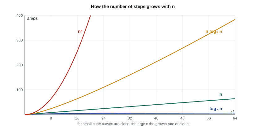
Suppose an algorithm performs f(n) basic steps on an input of size n. For large n, the term of f that grows fastest dominates everything else. If f(n) = 3n² + 20n + 100, then at n = 10 the three terms are 300, 200 and 100, all comparable; at n = 10,000 they are 300 million, 200,000 and 100, and the first term is more than 99.9 percent of the total. Constant factors like the 3 matter in practice, but they change with the machine and the compiler, while the n² does not. Asymptotic analysis keeps only the dominant term and drops its constant: f(n) grows like n².
| Growth rate | Name | Typical example | Steps at n = 1,000 | Steps at n = 1,000,000 |
|---|---|---|---|---|
| 1 | Constant | Read an array element by index | 1 | 1 |
| log₂ n | Logarithmic | Binary search in a sorted array | about 10 | about 20 |
| n | Linear | Linear search, summing an array | 1,000 | 1,000,000 |
| n log₂ n | Linearithmic | Merge sort, heapsort | about 10,000 | about 20 million |
| n² | Quadratic | Comparing every pair, insertion sort | 1 million | 10¹² |
| 2ⁿ | Exponential | Trying every subset | about 10³⁰¹ | beyond astronomical |
Big-O, Big-Omega and Big-Theta
The formal definitions make the idea precise. We say f(n) is O(g(n)), read as f is big-O of g, if there are positive constants c and n₀ such that f(n) ≤ c·g(n) for every n ≥ n₀. In words: beyond some starting point, f never grows faster than a constant multiple of g. Big-O is an upper bound. The definition deliberately ignores small inputs, through n₀, and constant factors, through c.
Two companions complete the set. f(n) is Ω(g(n)), big-Omega, if f(n) ≥ c·g(n) for some positive c and all large n: a lower bound. f(n) is Θ(g(n)), big-Theta, if it is both O(g(n)) and Ω(g(n)): g is a tight description of how f grows. Strictly, a linear search is O(n²) as well as O(n), because n² is also an upper bound, just a useless one. In everyday engineering conversation people say O when they mean Θ, and quote the tightest bound they know. In this course, when we say an operation is O(n) we mean that its cost grows linearly, no faster and, in the case discussed, no slower.
Worked problem
Proving a bound from the definition
Jonah's duplicate check makes f(n) = 3n² + 20n + 100 basic steps on a day's list of n records. Show that f(n) is O(n²) by finding constants c and n₀.
Show solution
- For n ≥ 1, each lower-order term is at most a multiple of n².
- \[20n \le 20n^2 \quad\text{and}\quad 100 \le 100n^2 \quad (n \ge 1)\]
- Add the three terms.
- \[f(n) = 3n^2 + 20n + 100 \le 3n^2 + 20n^2 + 100n^2 = 123n^2\]
- So the definition holds with c = 123 and n₀ = 1. A smaller c works for larger n₀: for n ≥ 20, 20n ≤ n² and 100 ≤ n², so f(n) ≤ 5n².
- \[f(n) \le 5n^2 \quad (n \ge 20)\]
Answer: f(n) = O(n²), with c = 123 and n₀ = 1, or c = 5 and n₀ = 20. Since f(n) ≥ 3n² as well, f(n) = Θ(n²).
Rules for analyzing code
You rarely need the formal definition once you know a few rules. A sequence of statements costs the sum of their costs, and the largest term wins: an O(n) loop followed by an O(n²) loop is O(n²). A loop costs the number of iterations times the cost of its body: a loop over n items with a constant-time body is O(n). Nested loops multiply: a loop over n items inside another loop over n items is O(n²). A function call costs whatever the function costs. Constant factors disappear, so a loop that runs 3n times is still O(n), and so are two separate passes over the data.
Logarithms appear whenever an algorithm repeatedly cuts the problem by a constant fraction. If each step halves the remaining range, then after k steps the range is n/2ᵏ, and the algorithm stops when that reaches 1, after k = log₂ n steps. Binary search, which compares the target with the middle element of a sorted array and discards half of it, is the standard example. Searching a sorted list of a million timestamps takes at most 20 comparisons; a billion takes 30. The base of the logarithm does not matter inside Big-O, because logarithms to different bases differ only by a constant factor, so we simply write O(log n).
# Binary search on sorted timestamps, counting comparisons
def binary_search(a, target):
    lo, hi, steps = 0, len(a) - 1, 0
    while lo <= hi:
        mid = (lo + hi) // 2
        steps += 1
        if a[mid] == target:
            return mid, steps
        if a[mid] < target:
            lo = mid + 1
        else:
            hi = mid - 1
    return -1, steps

for n in (1_000, 1_000_000, 1_000_000_000):
    a = range(0, 2 * n, 2)          # n sorted even numbers, not stored in memory
    worst = max(binary_search(a, t)[1] for t in (0, 2 * n - 2, -1, 2 * n))
print(f"n = {n:>13,}: at most {worst} comparisons")n = 1,000: at most 10 comparisons n = 1,000,000: at most 20 comparisons n = 1,000,000,000: at most 30 comparisons
The program uses a Python range object, which behaves like a sorted sequence without storing a billion numbers, and confirms that the number of steps grows by only about 10 each time n grows a thousandfold. That is what a logarithmic growth rate means in practice. The comparison with linear search is dramatic: for a billion items, 30 comparisons instead of up to a billion. The price is that the data must be kept sorted, which costs something when new items arrive. Much of this course is about structures, such as balanced search trees, that keep data in an order that supports fast searching while still allowing cheap insertion.
Back to the duplicate check
Jonah's duplicate check had two nested loops: for each of the m records in a new batch, scan all n records already stored for the day. That is O(m·n). With batches of a few hundred and n growing to 40,000 over the day, the late-afternoon uploads made millions of comparisons each, and the total work over the whole day grew roughly with the square of the day's record count. The fix is not a faster loop but a different structure. If the stored records' identifiers, a node serial number plus a timestamp, are kept in a hash set, each membership test costs O(1) on average, and checking a batch of m records costs O(m) regardless of how many records are already stored. Lesson 10 explains how a hash set achieves that.
# Duplicate check: nested scan versus a set, counting basic steps
import random
random.seed(7)

day = random.sample(range(10_000_000), 40_000)       # record ids stored so far today
batch = random.sample(day, 150) + random.sample(range(10_000_000, 10_000_150), 150)

steps = 0
dups_scan = 0
for r in batch:                 # O(m * n): compare with every stored id
    for s in day:
        steps += 1
        if r == s:
            dups_scan += 1
            break
print(f"nested scan: {dups_scan} duplicates found in {steps:,} comparisons")

stored = set(day)               # built once, kept up to date as records arrive
dups_set = sum(1 for r in batch if r in stored)   # O(m) on average
print(f"hash set: {dups_set} duplicates found in {len(batch)} lookups")nested scan: 150 duplicates found in 9,219,746 comparisons hash set: 150 duplicates found in 300 lookups
The nested scan finds the same 150 duplicates as the set, but it makes millions of comparisons where the set makes 300 lookups. The set has its own costs, about 40,000 entries of memory and the time to keep it up to date as records arrive, but on a server those costs are small and constant per record. This pattern, replacing a repeated search with a better structure, is the single most common performance fix in practice, and it is almost always worth more than tuning the inner loop.
What Big-O hides
Asymptotic analysis is powerful, but it hides things that matter in engineering. Constant factors are one: an O(n) algorithm with a constant of 1,000 loses to an O(n²) algorithm with a constant of 1 for every n below 1,000. Small inputs are another: for a list of eight items, a simple linear scan usually beats a clever logarithmic structure, which is why good library sort routines switch to insertion sort for short runs. Memory behavior is a third: two O(n) loops can differ several-fold in speed because one walks memory in order and the other jumps around. Finally, Big-O describes growth, not absolute time; it tells you that doubling n will roughly quadruple the time of an O(n²) algorithm, not how many milliseconds either will take.
For an embedded engineer there is one more caution. On the NS-4, n is often small and fixed: four lanes, sixteen vehicle classes, a 2,048-record buffer. What matters there is the worst-case number of cycles for that fixed n, measured or calculated precisely, because the radar interrupt must be serviced within a few microseconds. Big-O still guides the design, ruling out structures whose cost grows with the buffer size inside the interrupt handler, but the final check is a cycle count on the real processor. Maren's team measures worst-case execution time by toggling a spare output pin at the start and end of each routine and watching it on an oscilloscope, exactly as ELE-280 describes.
Common mistakes
MistakeKeeping constants and lower-order terms in a Big-O statement, such as O(3n² + 20n).
InsteadWrite the dominant term without its constant: O(n²). Discuss constants separately when they matter.
MistakeAssuming two nested loops are always O(n²).
InsteadMultiply the actual iteration counts. A loop over m inside a loop over n is O(m·n), and an inner loop that halves its range each time may be O(log n).
MistakeThinking an O(log n) algorithm is always faster than an O(n) one.
InsteadBig-O describes growth for large n. For small inputs, constants and memory behavior can make the simpler algorithm faster.
MistakeFixing a slow algorithm by tuning the inner loop.
InsteadCheck the growth rate first. Replacing a repeated search with a better structure usually helps far more than any micro-optimization.
MistakeUsing Big-O alone to argue that real-time code meets its deadline.
InsteadMeasure or calculate the worst-case cycles for the actual input size on the actual processor.
Summary and key terms
- Asymptotic analysis describes how cost grows with input size n, keeping only the dominant term and ignoring constant factors.
- f(n) = O(g(n)) means f grows no faster than a constant multiple of g for large n; Ω gives a lower bound and Θ a tight bound.
- Sequences add, loops multiply iteration count by body cost, nested loops multiply, and repeated halving gives a logarithm.
- The common growth rates are 1, log n, n, n log n, n² and 2ⁿ; the gaps between them become enormous for large n.
- Big-O hides constants, small-input behavior and memory effects, so measure real performance when it matters.
- Asymptotic analysis
- Describing how an algorithm's cost grows as the input size becomes large.
- Big-O
- An upper bound on growth: f(n) ≤ c·g(n) for all n beyond some n₀.
- Big-Omega
- A lower bound on growth: f(n) ≥ c·g(n) for all large n.
- Big-Theta
- A tight bound: f grows at the same rate as g, both above and below.
- Logarithmic time
- Cost that grows with log n, typical of algorithms that repeatedly halve the problem.
- Quadratic time
- Cost that grows with n², typical of algorithms that compare every pair of items.
- Binary search
- Searching a sorted array by repeatedly comparing with the middle element and discarding half.
Practice problems
Work each problem on paper first, then reveal the answer to check.
Give the Big-O of f(n) = 7n log n + 4n + 50.
Show answer
O(n log n).
A loop runs over n items, and for each item calls a function that does a binary search on a sorted array of n items. What is the total cost?
Show answer
O(n log n).
An O(n²) algorithm takes 2 s for n = 10,000. Estimate the time for n = 40,000.
Show answer
Four times n gives sixteen times the work: about 32 s.
How many comparisons does binary search need at most for 4 million sorted items?
Show answer
About log₂(4 × 10⁶) ≈ 22.
Show that 5n + 30 is O(n) by giving c and n₀.
Show answer
For n ≥ 30, 30 ≤ n, so 5n + 30 ≤ 6n: c = 6, n₀ = 30 (or c = 35, n₀ = 1).
Lesson quiz · 5 questions
Score 60% or more to complete this lesson.
Create a free account to save your progress, take quizzes and earn a certificate.