
CMP-200 · Lesson 12 of 12 · 23 min
Searching, graphs and a capstone design
The final lesson brings the course together. It starts with searching, the operation that most data structures exist to make fast, and refines the binary search of lesson 2 into the forms engineers actually use. It then introduces graphs, the most general structure in the course, which model anything made of connections: roads, networks, circuits, task dependencies and social links. Breadth-first and depth-first search, the two basic ways to explore a graph, reuse the queue and stack of lesson 5. Finally, a capstone design walks through the choice of every data structure in a complete system, the NS-4 node and the Northway server, the way Maren expects Jonah to present it at the end of his co-op term.
Searching revisited
Three search strategies cover almost every case. Linear search, O(n), works on any sequence, sorted or not, and is the right choice for small collections, for data searched only once, and for linked lists, which cannot be indexed. Binary search, O(log n), needs a sorted array and repays the cost of sorting when the same data is searched many times. Hashing, O(1) on average, answers exact-match questions fastest but cannot answer ordered ones. When the data changes often and ordered questions matter, a balanced search tree, O(log n) for everything, is the compromise. The skill is matching the strategy to the questions asked and how often the data changes.
Binary search is famous for being easy to describe and hard to write correctly. Jon Bentley reported that when he asked professional programmers to write it, most versions contained bugs, and a bug in the standard Java library's binary search, an overflow when computing the midpoint as (lo + hi)/2 for arrays of more than a billion elements, went unnoticed for nearly a decade until 2006. The robust form uses lo + (hi − lo)/2 for the midpoint in languages with fixed-size integers. The most useful variant in practice is not the search for an exact key but the lower bound: the first position whose key is greater than or equal to a target. It answers the questions that matter in real systems, such as where a new item should be inserted to keep the array sorted, and which is the first record at or after 17:00. Python provides it as bisect.bisect_left.
# Lower bound: the first index whose timestamp is >= target (bisect_left), with a range query
import bisect

def lower_bound(a, target):
    lo, hi = 0, len(a)                     # search the half-open range [lo, hi)
    while lo < hi:
        mid = lo + (hi - lo) // 2          # avoids overflow in fixed-size integer languages
        if a[mid] < target:
            lo = mid + 1
        else:
            hi = mid
    return lo

ts = [61200, 61230, 61275, 61300, 61300, 61345, 61410, 61500, 61620]   # seconds of day, sorted
for target in (61300, 61301, 61000, 62000):
    i = lower_bound(ts, target)
    assert i == bisect.bisect_left(ts, target)
    print(f"first record at or after {target}: index {i}")

lo, hi = lower_bound(ts, 61250), lower_bound(ts, 61420)
print("records in [61250, 61420):", ts[lo:hi])first record at or after 61300: index 3 first record at or after 61301: index 5 first record at or after 61000: index 0 first record at or after 62000: index 9 records in [61250, 61420): [61275, 61300, 61300, 61345, 61410]
Writing the search over the half-open range [lo, hi), where hi is one past the last candidate, removes most of the off-by-one errors: the loop runs while the range is non-empty, and every iteration shrinks it, so termination is clear. Two lower-bound searches then give any range query on a sorted array in O(log n + k), as the last line shows, with no tree at all. For data that is loaded once and queried many times, such as last year's records on the server, a sorted array with lower-bound searches uses less memory and is faster in practice than a search tree.
Graphs
A graph G = (V, E) consists of a set V of vertices, also called nodes, and a set E of edges, each joining a pair of vertices. In an undirected graph an edge works both ways, like a two-way street; in a directed graph each edge has a direction, like a one-way street or a dependency from one task to another. Edges may carry weights, such as distances or travel times. Two vertices joined by an edge are adjacent, and the number of edges at a vertex is its degree. A path is a sequence of vertices joined by edges, a cycle is a path that returns to its start, and a graph is connected if there is a path between every pair of vertices. Trees, from lesson 7, are exactly the connected graphs with no cycles.
Northway's interest in graphs is practical. The city of each deployment is modeled as a road graph: intersections are vertices and road segments between them are edges, with NS-4 nodes installed on some segments. When a node goes offline, the server must find which neighboring nodes can estimate its traffic, which is a question about adjacency. When a technician's van must visit several faulty nodes, the route is a question about paths. And when two nodes record the same transponder, the travel time between them only makes sense if the road graph connects them without passing a third node.
Representing a graph
There are two standard representations. An adjacency matrix is a V × V array whose entry [u][v] is 1, or the edge weight, if there is an edge from u to v, and 0 otherwise. It answers is there an edge from u to v in O(1), but it uses O(V²) memory and listing a vertex's neighbors takes O(V) time, even if it has only two. An adjacency list keeps, for each vertex, a list of its neighbors; it uses O(V + E) memory, lists the neighbors of v in time proportional to its degree, and tests for a particular edge in O(degree). Road networks, like most real graphs, are sparse: an intersection joins three or four roads, so E is a small multiple of V, and the adjacency list is the right choice. Dense graphs, where most pairs are connected, favor the matrix.
Worked problem
Memory for two representations
Ann Arbor's road graph for the deployment has 2,400 intersections and 3,300 two-way road segments. Estimate the memory for an adjacency matrix of 1-byte entries and for an adjacency list that stores each neighbor as a 4-byte vertex number plus a 4-byte weight, ignoring small per-list overheads.
Show solution
- The matrix has one entry for every ordered pair of vertices.
- \[V^2 = 2400^2 = 5\,760\,000 \text{ bytes} \approx 5.8 \text{ MB}\]
- In an undirected adjacency list each segment appears twice, once in each endpoint's list.
- \[2E = 2 \times 3300 = 6600 \text{ entries}\]
- \[6600 \times 8 = 52\,800 \text{ bytes} \approx 53 \text{ KB}\]
- \[\frac{5\,760\,000}{52\,800} \approx 109\]
Answer: About 5.8 MB for the matrix and 53 KB for the list, a factor of about 110. Almost all of the matrix's entries would be zero, because each intersection connects to only a few others.
Breadth-first search
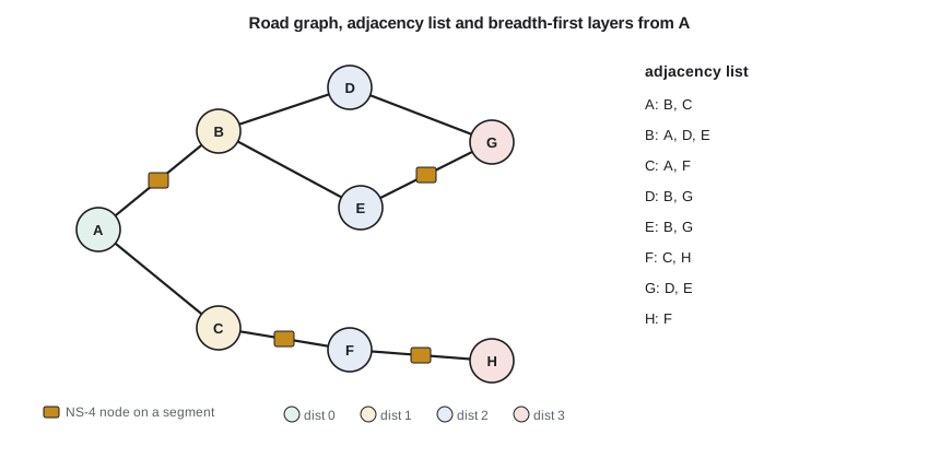
Breadth-first search, BFS, explores a graph outward from a starting vertex in layers: first the start, then all vertices one edge away, then all vertices two edges away, and so on. It uses a queue. Put the start in the queue and mark it visited; then, while the queue is not empty, dequeue a vertex and enqueue each of its unvisited neighbors, marking them visited as they are enqueued. Because vertices leave the queue in order of their distance from the start, BFS finds the shortest path, counted in edges, from the start to every reachable vertex, and recording each vertex's parent lets that path be traced back. Every vertex is enqueued once and every edge examined once or twice, so BFS costs O(V + E) with an adjacency list. Its main uses are shortest paths in unweighted graphs, finding everything within k steps, and testing whether a graph is connected.
Depth-first search
Depth-first search, DFS, goes as deep as it can along one path before backing up to try another, like exploring a maze by keeping one hand on the wall. It is naturally recursive: visit a vertex, mark it, and recursively visit each unvisited neighbor; or, iteratively, use an explicit stack in place of BFS's queue, as lesson 6 described. DFS also costs O(V + E). It does not find shortest paths, but it is the basis of many algorithms: detecting cycles, finding connected components, ordering tasks so that each comes after the tasks it depends on (topological sort), and finding the bridges whose loss would split a network. On large graphs, recursive DFS can run thousands of levels deep, so production code uses the explicit stack.
# BFS for hop distances and paths in a road graph, and DFS to find connected components
from collections import deque

roads = [("A","B"),("A","C"),("B","D"),("B","E"),("C","F"),("E","G"),("F","H"),("D","G"),
         ("X","Y")]                       # X-Y is a separate rural segment
adj = {}
for u, v in roads:                        # undirected adjacency list
    adj.setdefault(u, []).append(v)
    adj.setdefault(v, []).append(u)

def bfs(start):
    dist, parent, q = {start: 0}, {start: None}, deque([start])
    while q:
        u = q.popleft()
        for w in adj[u]:
            if w not in dist:
                dist[w], parent[w] = dist[u] + 1, u
                q.append(w)
    return dist, parent

def path(parent, v):
    out = []
    while v is not None:
        out.append(v); v = parent[v]
    return out[::-1]

dist, parent = bfs("A")
print("hops from A:", dict(sorted(dist.items())))
print("path A to H:", " -> ".join(path(parent, "H")))

def components():
    seen, comps = set(), []
    for s in sorted(adj):
        if s in seen: continue
        stack, comp = [s], []
        seen.add(s)
        while stack:                      # iterative DFS with an explicit stack
            u = stack.pop(); comp.append(u)
            for w in adj[u]:
                if w not in seen:
                    seen.add(w); stack.append(w)
        comps.append(sorted(comp))
    return comps

print("connected components:", components())hops from A: {'A': 0, 'B': 1, 'C': 1, 'D': 2, 'E': 2, 'F': 2, 'G': 3, 'H': 3}
path A to H: A -> C -> F -> H
connected components: [['A', 'B', 'C', 'D', 'E', 'F', 'G', 'H'], ['X', 'Y']]The output shows BFS's layers from intersection A and the shortest path to H, and DFS finding two connected components: the city network and the separate rural segment X to Y. If an NS-4 on the rural segment reports a transponder that was also seen in the city, the server knows at once that the travel time cannot be computed from the road graph it holds. Finding shortest paths by distance or travel time rather than by number of edges needs Dijkstra's algorithm, which replaces BFS's queue with the priority queue of lesson 9; it, minimum spanning trees and the other weighted graph algorithms are the subject of CMP-301 and CMPUT-204.
Capstone: choosing the structures for a system
Maren asks Jonah to finish his term by presenting the data-structure design of the whole NS-4 system in one table, justifying each choice from the operations it serves, as lesson 1 taught. His table is below. Read it as a summary of the course: every structure appears, and every choice follows from listing the operations, their frequency, the data size and the constraints of the machine they run on.
| Data | Where | Operations and constraints | Structure | Cost of the key operations |
|---|---|---|---|---|
| Radar detections | Node, interrupt to main loop | Append in an interrupt, remove in order, no locks, fixed RAM | Ring buffer (lesson 5) | O(1) push and pop |
| Vehicle records awaiting upload | Node | Append up to 50 per second, remove oldest after upload, 24 KB | Circular array of 12-byte records (lessons 3, 5) | O(1) |
| Pending events | Node | Raise and clear in any order, from interrupts, no heap | Doubly linked list in a fixed pool (lesson 4) | O(1) add and clear |
| Modem messages | Node | Most urgent first, oldest first within a class | Binary min-heap of 16 descriptors (lesson 9) | O(log n) insert and remove |
| Vehicle classification rules | Node, flash | Walk one path per vehicle, replace as data | Decision tree stored as an array (lesson 7) | At most tree height, 5 tests |
| Transponder sightings | Node | Look up by 16-bit id, insert, evict old, 6 KB | Open-addressing hash table, linear probing (lesson 10) | O(1) average, α < 0.7 |
| Speed percentiles | Node | 85th percentile of up to 900 speeds per period | Histogram of 251 counters (lesson 11) | O(n + k), no sorting |
| Node status by serial number | Server | Exact lookup on every upload | Hash table (dict) (lesson 10) | O(1) average |
| Duplicate record check | Server | Membership test for each new record | Hash set (lessons 2, 10) | O(1) average per record |
| Records by time | Server, database | Range and successor queries over years of data | B+ tree index (lesson 8) | O(log n + k) |
| Daily top speeds | Server | Largest 100 of about 30 million, streamed | Size-k min-heap (lesson 9) | O(n log k) |
| Nightly export | Server | Sort 30 million records by node and time | External merge sort (lesson 11) | O(n log n) |
| Road network | Server | Neighbors, hop distances, connectivity | Adjacency list with BFS and DFS (lesson 12) | O(V + E) |
Two patterns stand out in the table. On the node, every structure has a fixed size chosen at design time, every operation has a small constant or logarithmic worst case, and none uses the heap or recursion, because the node must run unattended for years and meet its timing in the worst case. On the server, the structures grow with the data, and the choices aim at average-case speed and at keeping the growth rate down as the deployment expands from one city to many. The same problem, storing and finding vehicle records, gets different answers in different places, which is the whole point of the course: there is no best data structure, only the best one for a given set of operations on a given machine.
Jonah's presentation also lists what he would test. Each fixed-size structure gets a stress test at its capacity, with drop counters to show whether the limits are ever reached in a simulated rush hour. Each hash table gets a test with real serial numbers and transponder identifiers to confirm the keys spread evenly. The server's routines get tests at ten times today's data volume, to confirm that their growth rates hold, the lesson from his duplicate-check bug in week two. And every routine that runs in an interrupt gets a worst-case timing measurement on the real processor with an oscilloscope, because asymptotic analysis guides the design but measurement confirms it.
Common mistakes
MistakeComputing a binary search midpoint as (lo + hi) / 2 with fixed-size integers.
InsteadUse lo + (hi − lo) / 2 so the sum cannot overflow on very large arrays.
MistakeMarking a vertex visited only when it is dequeued in BFS.
InsteadMark it when it is enqueued, or the same vertex can be added to the queue many times.
MistakeUsing an adjacency matrix for a large sparse graph such as a road network.
InsteadAn adjacency list uses O(V + E) memory instead of O(V²) and lists neighbors in proportion to the degree.
MistakeExpecting DFS to find shortest paths.
InsteadDFS finds a path, not the shortest; BFS finds shortest paths in unweighted graphs and Dijkstra's algorithm in weighted ones.
MistakeChoosing data structures without stating the operations, sizes and machine constraints.
InsteadWrite those down first; the same data can need different structures on a microcontroller and on a server.
Summary and key terms
- Linear search suits small or unsorted data, binary search suits sorted arrays searched often, and hashing suits exact-match lookups.
- The lower-bound form of binary search finds insertion points and supports range queries on sorted arrays in O(log n + k).
- A graph is a set of vertices joined by edges; sparse graphs are stored as adjacency lists and dense ones as matrices.
- BFS explores in layers with a queue and finds shortest paths by edge count; DFS goes deep with a stack and finds components and cycles; both cost O(V + E).
- Good system design matches each data structure to its operations, data size and the constraints of the machine it runs on.
- Lower bound (search)
- The first position in a sorted array whose key is greater than or equal to a target.
- Graph
- A set of vertices together with a set of edges joining pairs of vertices.
- Adjacency list
- A graph representation that stores, for each vertex, the list of its neighbors.
- Adjacency matrix
- A V × V array recording whether, or with what weight, each pair of vertices is joined.
- Breadth-first search
- Exploring a graph in order of distance from the start, using a queue.
- Depth-first search
- Exploring a graph by following each path as deep as possible before backing up, using a stack or recursion.
- Connected component
- A maximal set of vertices in which every pair is joined by some path.
Practice problems
Work each problem on paper first, then reveal the answer to check.
In the sorted array [3, 5, 5, 8, 12], what does the lower bound of 5 return, and of 6?
Show answer
Index 1 for 5; index 3 for 6.
An undirected graph has 10,000 vertices and 25,000 edges. How many entries does its adjacency list hold?
Show answer
2 × 25,000 = 50,000 neighbor entries.
Run BFS from A on edges A–B, A–C, B–D, C–D, D–E. What is the hop distance to E?
Show answer
A 0, B and C 1, D 2, E 3.
Which search would you use to check whether removing one road splits a city's network into two parts?
Show answer
Depth-first search, the basis of the bridge-finding algorithm.
Why does the NS-4 avoid the heap and recursion while the server uses both freely?
Show answer
The node must meet worst-case timing and memory limits unattended for years; the server has ample memory and aims at average speed.
Lesson quiz · 5 questions
Score 60% or more to complete this lesson.
Create a free account to save your progress, take quizzes and earn a certificate.