
CMP-200 · Lesson 11 of 12 · 24 min
Sorting algorithms
Sorting puts items into order, and it is one of the most studied problems in computing because so much else depends on it. Sorted data can be searched with binary search, merged with other sorted data in linear time, scanned for duplicates in one pass, divided into percentiles and displayed in a form people can read. Databases sort to answer ORDER BY and to build indexes; graphics systems sort objects by depth; compression programs sort to find repeated patterns. This lesson covers the simple quadratic sorts and why they still matter, the two great divide-and-conquer sorts, merge sort and quicksort, the properties that distinguish sorting algorithms, and the non-comparison sorts that beat the usual limits when keys are small integers. CMPUT-204 proves the lower bounds formally; here the focus is on how the algorithms work, what they cost and how to choose between them on real hardware.
Jonah has two sorting jobs. On the server, each night's export of vehicle records must be sorted by node and then by timestamp, about 30 million records, before analysts load it. On the NS-4, the firmware computes the 85th-percentile speed of each lane every fifteen minutes, a standard traffic engineering measure used to set speed limits, which means sorting the up to 900 speeds recorded in that period. The two jobs differ by a factor of thirty thousand in size and run on machines that differ even more in memory, so they need different algorithms.
Properties of sorting algorithms
Besides speed, three properties decide which sort to use. A sort is stable if items with equal keys keep their original relative order. Stability matters whenever you sort by one key after another: to get records ordered by node and, within each node, by timestamp, you can sort by timestamp first and then stably by node, and the timestamp order survives within each node. A sort is in place if it needs only a constant amount, or at most O(log n), of extra memory beyond the array itself; that matters on the NS-4. And a sort is adaptive if it runs faster on input that is already nearly sorted, which real data often is: records arrive mostly in timestamp order, with only retried uploads out of place.
Insertion sort
Insertion sort builds a sorted prefix one item at a time. For each new item, it shifts the larger items of the sorted prefix one place right and drops the new item into the gap, much as a card player sorts a hand. In the worst case, input in reverse order, each new item moves past all the earlier ones, giving about n²/2 comparisons and moves, O(n²). But insertion sort is stable, in place, simple, and strongly adaptive: on input that is already sorted it makes only n − 1 comparisons, and on nearly sorted input its cost is O(n + d), where d is the number of out-of-order pairs. For small arrays, up to a few dozen items, its tiny constant factor makes it faster than the asymptotically better algorithms, which is why good library sorts switch to insertion sort for small subarrays. Selection sort and bubble sort are also O(n²) but lack insertion sort's adaptivity, and have no practical advantage over it.
# Insertion sort, counting comparisons, on random, sorted and nearly sorted speeds
import random

def insertion_sort(a):
    a, comps = list(a), 0
    for i in range(1, len(a)):
        x, j = a[i], i - 1
        while j >= 0:
            comps += 1
            if a[j] <= x:
                break
            a[j + 1] = a[j]
            j -= 1
        a[j + 1] = x
    return a, comps

random.seed(3)
n = 900
speeds = [round(random.uniform(40, 130), 1) for _ in range(n)]
nearly = sorted(speeds)
for _ in range(20):                         # 20 random swaps of adjacent items
    i = random.randrange(n - 1)
    nearly[i], nearly[i + 1] = nearly[i + 1], nearly[i]

for name, data in (("random", speeds), ("sorted", sorted(speeds)), ("nearly sorted", nearly)):
    out, c = insertion_sort(data)
    assert out == sorted(data)
print(f"{name:>13}: {c:>7,} comparisons (n^2/4 = {n * n // 4:,})") random: 207,147 comparisons (n^2/4 = 202,500)
sorted: 899 comparisons (n^2/4 = 202,500)
nearly sorted: 911 comparisons (n^2/4 = 202,500)Merge sort
Merge sort, described by John von Neumann in 1945, is the clearest example of divide and conquer. Split the array into two halves, sort each half recursively, and merge the two sorted halves into one sorted array. Merging is the heart of it: keep a pointer at the front of each half, repeatedly copy the smaller front item to the output and advance that pointer, and when one half runs out copy the rest of the other. Merging n items takes at most n − 1 comparisons. The recursion goes log₂ n levels deep, and each level merges a total of n items, so merge sort costs O(n log n) in every case, best, average and worst, as the recurrence T(n) = 2T(n/2) + cn from lesson 6 predicts.
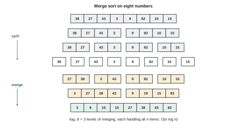
Merge sort is stable, provided the merge takes from the left half when the front items are equal, and its O(n log n) worst case makes it predictable. Its drawback is memory: merging needs a temporary array of n items, so it is not in place. On a server with gigabytes of memory that is acceptable, and merge sort's sequential access pattern suits caches well. Merge sort is also the natural algorithm for data too large for memory, external sorting: sort chunks that fit in memory, write each sorted chunk to disk, then merge all the chunks in one streaming pass using a min-heap of the chunks' front items, the priority queue of lesson 9. That is exactly how Northway's nightly export sorts 30 million records with a few hundred megabytes of memory.
Worked problem
Counting the cost of merge sort
Estimate the comparisons merge sort makes on the 30 million records of the nightly export, and compare with insertion sort's worst case. Then estimate the time for each at 100 million comparisons per second.
Show solution
- Merge sort makes at most about n log₂ n comparisons.
- \[n\log_2 n = 3\times10^7 \times \log_2(3\times10^7) \approx 3\times10^7 \times 24.8 \approx 7.4\times10^8\]
- \[t_{\text{merge}} \approx \frac{7.4\times10^8}{10^8\ \text{s}^{-1}} \approx 7.4 \text{ s}\]
- Insertion sort's worst case is about n²/2 comparisons.
- \[\frac{n^2}{2} = \frac{(3\times10^7)^2}{2} = 4.5\times10^{14}\]
- \[t_{\text{insertion}} \approx \frac{4.5\times10^{14}}{10^8\ \text{s}^{-1}} = 4.5\times10^6 \text{ s} \approx 52 \text{ days}\]
Answer: About 7 seconds for merge sort against roughly 52 days for insertion sort in the worst case. Growth rate, not processor speed, decides which sorts are usable at this scale.
Quicksort
Quicksort, invented by Tony Hoare in 1959, is also divide and conquer but does its work before the recursion rather than after. Choose an item called the pivot, and partition the array so that every item smaller than the pivot comes before it and every larger item after it; the pivot is then in its final position. Recursively sort the two parts. Partitioning is done in place in one linear pass, swapping items across a moving boundary, so quicksort needs no temporary array, only the recursion stack. When the pivot splits the array roughly in half, quicksort makes about 1.39·n log₂ n comparisons and runs very fast, because its inner loop is tiny and walks memory sequentially. On random data it is usually the fastest general-purpose comparison sort.
Quicksort's weakness is its worst case. If the pivot is always the smallest or largest item, each partition removes only one item, the recursion goes n levels deep and the cost is O(n²). Naively choosing the first item as the pivot produces exactly this worst case on input that is already sorted, the commonest kind of real input. Practical implementations avoid it by choosing the pivot as the median of three items, or at random, which makes the bad case vanishingly unlikely; by recursing on the smaller part first and looping on the larger, which bounds the stack depth at O(log n); and by switching to heapsort if the recursion gets too deep, which bounds the worst case at O(n log n). That combination, introsort, is what the C++ standard library's std::sort uses. Quicksort is in place but not stable.
# Quicksort with median-of-three pivots versus a naive first-element pivot, on sorted input
import sys
sys.setrecursionlimit(10_000)
comps = 0

def partition(a, lo, hi, pick):
    global comps
    p = pick(a, lo, hi)
    a[p], a[hi] = a[hi], a[p]               # move the pivot to the end
    pivot, i = a[hi], lo
    for j in range(lo, hi):
        comps += 1
        if a[j] < pivot:
            a[i], a[j] = a[j], a[i]
            i += 1
    a[i], a[hi] = a[hi], a[i]
    return i

def quicksort(a, lo, hi, pick):
    while lo < hi:
        p = partition(a, lo, hi, pick)
        if p - lo < hi - p:                 # recurse on the smaller side, loop on the larger
            quicksort(a, lo, p - 1, pick); lo = p + 1
        else:
            quicksort(a, p + 1, hi, pick); hi = p - 1

first = lambda a, lo, hi: lo
def median3(a, lo, hi):
    mid = (lo + hi) // 2
    return sorted([(a[lo], lo), (a[mid], mid), (a[hi], hi)])[1][1]

for name, pick in (("first element", first), ("median of three", median3)):
    data = list(range(2000))                # already sorted
    comps = 0
    quicksort(data, 0, len(data) - 1, pick)
    assert data == sorted(data)
print(f"{name:>15} pivot on sorted input: {comps:>9,} comparisons")first element pivot on sorted input: 1,999,000 comparisons median of three pivot on sorted input: 17,964 comparisons
The limit for comparison sorts
Insertion sort, merge sort, quicksort and heapsort all learn about the order of the items only by comparing pairs. Any such comparison sort needs at least about log₂(n!) ≈ n log₂ n − 1.44n comparisons in the worst case, because there are n! possible orderings of n distinct items and each comparison can at best halve the number still possible. So no comparison sort can beat O(n log n), and merge sort and heapsort are asymptotically optimal. CMPUT-204 proves this bound with decision trees. The bound does not apply to algorithms that look at the keys themselves rather than only comparing them.
Counting sort and radix sort
When the keys are small integers, counting sort beats the bound. To sort n items whose keys lie between 0 and k − 1, count how many items have each key in an array of k counters, convert the counts to starting positions with a running sum, then place each item at its position, advancing that position. The cost is O(n + k) time and O(n + k) memory, and the sort is stable. Radix sort applies counting sort to one digit of the key at a time, from the least significant digit to the most, relying on stability so that each pass preserves the order from the passes before. Sorting 32-bit keys one byte at a time takes four passes of counting sort with 256 counters each, O(n) overall, and it is often the fastest way to sort large arrays of integers.
The NS-4's percentile job is a natural fit. Speeds are recorded in tenths of a km/h but only to the nearest 1 km/h for the percentile, and no speed exceeds 250 km/h, so there are only 251 possible keys. The firmware does not even need to sort: it keeps a histogram of 251 16-bit counters, 502 bytes, increments one counter per vehicle, and at the end of the period walks the histogram summing counts until it passes 85 percent of the total. That is counting sort with the final placement step left out, O(n + k) time, fixed memory, no comparisons and no recursion, a design that fits the microcontroller far better than any comparison sort.
Worked problem
The 85th-percentile speed from a histogram
In one fifteen-minute period, lane 2 recorded 400 vehicles. The cumulative histogram reaches 331 vehicles at 104 km/h and 344 vehicles at 105 km/h. Find the 85th-percentile speed, defined here as the speed at or below which at least 85 % of vehicles traveled.
Show solution
- The target count is 85 % of the total.
- \[0.85 \times 400 = 340\]
- Walk the cumulative histogram until the running count reaches 340.
- \[\text{count}(\le 104) = 331 < 340, \qquad \text{count}(\le 105) = 344 \ge 340\]
- The first speed at which the running count reaches the target is 105 km/h.
Answer: The 85th-percentile speed is 105 km/h, found in at most 251 steps over the histogram, independent of how many vehicles passed.
Choosing a sort
In practice you rarely write a sort from scratch on a server: Python's sorted and list.sort use Timsort, a hybrid of merge sort and insertion sort devised by Tim Peters in 2002, which is stable, O(n log n) in the worst case and exceptionally fast on real data that contains runs of already ordered items; Java uses it for objects too. C's qsort and C++'s std::sort are quicksort-based introsorts, fast but not stable; std::stable_sort is a merge sort. What you must know is which properties you need. Sorting by several keys needs stability. Huge data needs an external merge sort. Memory-starved firmware needs an in-place sort with a guaranteed bound, such as heapsort, or better, a counting approach that avoids sorting. Small or nearly sorted inputs favor insertion sort. And integer keys from a small range invite counting or radix sort.
| Algorithm | Best | Average | Worst | Extra memory | Stable | Adaptive |
|---|---|---|---|---|---|---|
| Insertion sort | O(n) | O(n²) | O(n²) | O(1) | Yes | Yes |
| Merge sort | O(n log n) | O(n log n) | O(n log n) | O(n) | Yes | No (Timsort: yes) |
| Quicksort | O(n log n) | O(n log n) | O(n²) | O(log n) stack | No | No |
| Heapsort | O(n log n) | O(n log n) | O(n log n) | O(1) | No | No |
| Counting sort | O(n + k) | O(n + k) | O(n + k) | O(n + k) | Yes | No |
| Radix sort (d digits) | O(d(n + k)) | O(d(n + k)) | O(d(n + k)) | O(n + k) | Yes | No |
Common mistakes
MistakeChoosing a pivot naively, such as the first element, in quicksort.
InsteadUse median of three or a random pivot; a first-element pivot is quadratic on sorted input.
MistakeSorting by a second key with an unstable sort after sorting by the first.
InsteadUse a stable sort, or sort once with a combined key such as (node, timestamp).
MistakeUsing an O(n²) sort for a large data set because it worked in testing.
InsteadTest with realistic sizes; quadratic sorts that take milliseconds on 1,000 items take hours on a million.
MistakeSorting a full array just to find a percentile of small integer values.
InsteadKeep a histogram (counting sort) or use a selection algorithm; full sorting is unnecessary work.
MistakeAssuming merge sort can run in place on a microcontroller.
InsteadStandard merge sort needs an O(n) buffer; use heapsort, insertion sort for small n, or a counting approach.
Summary and key terms
- Sorting algorithms differ in speed and in being stable, in place and adaptive.
- Insertion sort is O(n²) but fast for small or nearly sorted inputs, and is used inside hybrid sorts.
- Merge sort is a stable O(n log n) divide-and-conquer sort that needs O(n) extra memory and suits external sorting.
- Quicksort partitions in place around a pivot, is very fast on average, and needs good pivot choice to avoid O(n²).
- Comparison sorts need Ω(n log n) comparisons; counting and radix sort beat this for small integer keys.
- Stable sort
- A sort that keeps items with equal keys in their original relative order.
- In-place sort
- A sort that uses only a small, constant or logarithmic, amount of memory beyond the array.
- Merge
- Combining two sorted sequences into one sorted sequence in linear time.
- Pivot
- The item quicksort uses to partition the array into smaller and larger items.
- Comparison sort
- A sort that learns the order of items only by comparing pairs of keys.
- Counting sort
- A sort for small integer keys that counts each key's occurrences and places items by running sums.
- Timsort
- A stable hybrid of merge sort and insertion sort used by Python and Java that exploits existing runs.
Practice problems
Work each problem on paper first, then reveal the answer to check.
How many comparisons does insertion sort make on an already sorted array of 500 items?
Show answer
n − 1 = 499.
Merge sort runs on 1,048,576 items. How many levels of merging are there?
Show answer
log₂ 1,048,576 = 20.
Records must be ordered by lane, and by time within each lane. With a stable sort, which key do you sort by first?
Show answer
Time first, then lane, so the time order survives within each lane.
Counting sort is used on 10,000 items with keys from 0 to 99. What are its time and extra memory?
Show answer
O(n + k): about 10,100 steps and 100 counters plus an output array of 10,000.
Why does quicksort with a first-element pivot take O(n²) on sorted input?
Show answer
Each pivot is the smallest item, so each partition removes only one item and the recursion goes n levels deep.
Lesson quiz · 5 questions
Score 60% or more to complete this lesson.
Create a free account to save your progress, take quizzes and earn a certificate.