
CHE-460 · Lesson 9 of 12 · 18 min
Optimization with process models
The sensitivity analysis in lesson 8 showed that the ester column can meet its purity at many combinations of stages and reflux, and the purge study in lesson 7 showed a trade-off between propanol build-up and ethanol losses. Each of those is a decision with a cost on both sides. Priya, the cost engineer on the project, asks Theo for the combination that gives the lowest annual cost, so that the contractor can be told what to design for. That is an optimization problem, and process models are the natural tool for solving it.
Formulating an optimization problem
An optimization problem has four parts. The objective function is the quantity to minimize or maximize, such as total annual cost or profit. The decision variables are the inputs the optimizer may change, such as reflux ratio or purge fraction. The constraints are conditions that must hold, such as product purity at or above 99.7 %, or a vessel temperature below a limit. And the model connects the decision variables to the objective and constraints. A badly formulated problem gives a precise answer to the wrong question, so most of the engineering lies in the formulation.
For the ester column, Theo writes the objective as an equivalent annual cost: the steam cost for the reboiler, plus a capital charge on the column shell and the reboiler, plus the value of ethanol lost in the purge, plus a quality cost for the propanol held in the loop. The steam is priced at 12 dollars per gigajoule, Kingfisher Bioenergy's planning price, over 8,400 operating hours. The capital charge converts installed cost to an annual figure with a factor of 0.15 per year, a common approximation for capital recovery plus maintenance. The purity constraint is met by choosing the number of stages from the Gilliland relation for each reflux, so the column always meets its specification.
One variable: golden section search
With one decision variable, the reflux ratio, and a single minimum in the range, the golden section search is simple and robust. It brackets the minimum between two values, evaluates the objective at two interior points placed at the golden ratio, discards the part of the bracket that cannot contain the minimum, and repeats. Each step shrinks the bracket by a factor of 0.618 and needs only one new function evaluation. It needs no derivatives, which matters when each evaluation is a full simulation with its own convergence noise.
# Economic optimization of the ester column reflux and the recycle purge (illustrative costs, million per year)
import math
alpha, F, zF, xD, xB = 2.5, 63.8, 0.591, 0.985, 0.003
D = F * (zF - xB) / (xD - xB)
Nmin = math.log((xD / (1 - xD)) * ((1 - xB) / xB)) / math.log(alpha)
Rmin = (xD / zF - alpha * (1 - xD) / (1 - zF)) / (alpha - 1)
HOURS, STEAM, LAT = 8400, 12.0, 32.0          # h/yr, per GJ, kJ/mol of boil-up (illustrative)
def stages(R):
    X = (R - Rmin) / (R + 1)
    Y = 1 - math.exp((1 + 54.4 * X) / (11 + 117.2 * X) * (X - 1) / math.sqrt(X))
    return (Y + Nmin) / (1 - Y)
def propanol(p):            # propanol held in the recycle, kmol/h (from the lesson 7 balance)
    return 0.97 * 0.20 * (1 - p) / (1 - 0.97 * (1 - p))
def cost(R, p):
    if R <= Rmin * 1.01 or not (0 <= p < 0.5): return 1e9
    V = (R + 1) * D
    duty = V * LAT / 3600                                       # MW
    steam = duty * 3.6 * HOURS * STEAM / 1e6                    # million per year
    capital = 0.06 * stages(R) + 0.40 * (V / 89.4) ** 0.6       # million, installed (illustrative)
    annual_capital = 0.15 * capital                             # capital charge factor
    loss = p * 17.7 * 46.07 * HOURS * 0.90 / 1e6                # ethanol lost in the purge, million per year
    quality = 0.06 * propanol(p)                                # off-spec risk and extra stripping, million per year per kmol/h held
    return steam + annual_capital + loss + quality
# 1. Golden-section search on R with the purge fixed at 1 %
g = (math.sqrt(5) - 1) / 2
a, b = 1.1, 3.0
c, d = b - g * (b - a), a + g * (b - a)
for it in range(40):
    if cost(c, 0.01) < cost(d, 0.01): b, d = d, c; c = b - g * (b - a)
    else: a, c = c, d; d = a + g * (b - a)
Ropt = (a + b) / 2
print(f"golden section (purge 1 %): R_opt = {Ropt:.3f} = {Ropt / Rmin:.2f} Rmin, {stages(Ropt):.1f} stages, cost {cost(Ropt, 0.01):.4f} M/yr")
for R in (1.2, 1.3, Ropt, 1.6, 2.0):
    print(f"   R = {R:.3f}: stages {stages(R):5.1f}, total {cost(R, 0.01):.4f} M/yr")
# 2. Nelder-Mead on (R, p) together
def nelder_mead(f, x0, step, tol=1e-9, maxit=500):
    pts = [x0] + [ [x0[i] + (step[i] if j == i else 0) for i in range(len(x0))] for j in range(len(x0))]
    vals = [f(*p) for p in pts]
    for it in range(maxit):
        order = sorted(range(len(pts)), key=lambda i: vals[i]); pts = [pts[i] for i in order]; vals = [vals[i] for i in order]
        if vals[-1] - vals[0] < tol: break
        cen = [sum(p[i] for p in pts[:-1]) / (len(pts) - 1) for i in range(len(x0))]
        xr = [cen[i] + (cen[i] - pts[-1][i]) for i in range(len(x0))]; fr = f(*xr)
        if fr < vals[0]:
            xe = [cen[i] + 2 * (cen[i] - pts[-1][i]) for i in range(len(x0))]; fe = f(*xe)
            pts[-1], vals[-1] = (xe, fe) if fe < fr else (xr, fr)
        elif fr < vals[-2]: pts[-1], vals[-1] = xr, fr
        else:
            xc = [cen[i] + 0.5 * (pts[-1][i] - cen[i]) for i in range(len(x0))]; fc = f(*xc)
            if fc < vals[-1]: pts[-1], vals[-1] = xc, fc
            else:
                pts = [pts[0] ] + [ [pts[0][i] + 0.5 * (p[i] - pts[0][i]) for i in range(len(x0))] for p in pts[1:] ]
                vals = [f(*p) for p in pts]
    return pts[0], vals[0], it
(xR, xp), fbest, it = nelder_mead(cost, [1.8, 0.05], [0.2, 0.02])
print(f"Nelder-Mead: R = {xR:.3f}, purge = {100 * xp:.2f} %, cost {fbest:.4f} M/yr after {it} iterations")
print(f"   propanol held in the loop {propanol(xp):.2f} kmol/h")
# 3. Steepest descent with central-difference gradients on scaled variables u = (R, purge in %)
cu = lambda u0, u1: cost(u0, u1 / 100)
u = [1.8, 5.0]; h = 1e-4
for it in range(1, 201):
    gr = [(cu(u[0] + h, u[1]) - cu(u[0] - h, u[1])) / (2 * h), (cu(u[0], u[1] + h) - cu(u[0], u[1] - h)) / (2 * h)]
    t = 1.0
    while cu(u[0] - t * gr[0], u[1] - t * gr[1]) > cu(*u) - 1e-4 * t * (gr[0] ** 2 + gr[1] ** 2) and t > 1e-10: t /= 2
    u = [u[0] - t * gr[0], u[1] - t * gr[1] ]
if it in (1, 10, 50, 200): print(f"steepest descent step {it:3d}: R = {u[0]:.3f}, purge = {u[1]:.2f} %, cost {cu(*u):.4f} M/yr")golden section (purge 1 %): R_opt = 1.425 = 1.36 Rmin, 22.8 stages, cost 0.9176 M/yr R = 1.200: stages 27.8, total 0.9314 M/yr R = 1.300: stages 25.2, total 0.9211 M/yr R = 1.425: stages 22.8, total 0.9176 M/yr R = 1.600: stages 20.7, total 0.9222 M/yr R = 2.000: stages 17.9, total 0.9519 M/yr Nelder-Mead: R = 1.425, purge = 1.39 %, cost 0.9154 M/yr after 38 iterations propanol held in the loop 4.40 kmol/h steepest descent step 1: R = 1.724, purge = 4.96 %, cost 1.0248 M/yr steepest descent step 10: R = 1.436, purge = 4.58 %, cost 0.9974 M/yr steepest descent step 50: R = 1.425, purge = 3.15 %, cost 0.9462 M/yr steepest descent step 200: R = 1.425, purge = 1.44 %, cost 0.9154 M/yr
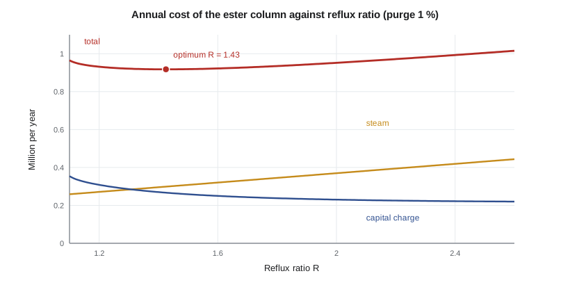
The golden section search finds an optimum reflux ratio of 1.425, or 1.36 times the minimum, with 22.8 theoretical stages and an annual cost of 0.918 million dollars. The cost curve is flat near the optimum: reflux ratios from 1.3 to 1.6 all cost within half a percent of the best. This flatness is typical of column optimization and is useful. It means the engineer can choose a reflux within that range for other reasons, such as operating margin or matching a standard column size, at almost no cost. The often-quoted rule that the optimum reflux lies between about 1.2 and 1.5 times the minimum reflects the same flat curve.
Several variables: Nelder-Mead and gradient methods
With two or more decision variables, other methods are needed. The Nelder-Mead simplex method, published in 1965, uses a simplex of \(n + 1\) points in \(n\) variables, and moves it by reflection, expansion, contraction and shrinking toward lower values of the objective. Like golden section, it needs no derivatives. It is robust for small problems with noisy objectives and widely used with simulators, though it can be slow for many variables and is not guaranteed to converge to a true minimum in all cases. Applied to reflux and purge together, it finds a reflux of 1.425 and a purge of 1.39 %, with an annual cost of 0.915 million dollars, in 38 iterations.
Gradient methods use derivatives of the objective to choose a direction. The simplest, steepest descent, steps in the direction of the negative gradient. It converges slowly when the objective is much more sensitive to one variable than another, as here, where cost depends strongly on reflux and weakly on purge. The code shows it: after 50 steps the reflux is right but the purge is still at 3.15 %; it takes 200 steps to reach the optimum. Scaling the variables so that they have similar effects helps, and practical gradient methods, such as quasi-Newton methods, build up curvature information to choose better directions.
Large process optimizations with many variables and constraints use sequential quadratic programming, SQP, which at each step solves a quadratic approximation of the objective with linearized constraints. It is the standard method in commercial simulators for constrained optimization, and in equation-oriented simulators, where derivatives are available analytically, it can handle thousands of variables. In sequential-modular simulators, derivatives are estimated by perturbing the flowsheet, which makes each iteration expensive and sensitive to convergence noise; the convergence tolerances of the flowsheet must be tighter than the perturbation steps.
| Method | Derivatives? | Variables | Notes |
|---|---|---|---|
| Golden section | No | One | Robust; needs a bracket with one minimum |
| Nelder-Mead simplex | No | Few | Robust to noise; can be slow |
| Steepest descent | Yes | Many | Slow with poorly scaled variables |
| Quasi-Newton | Yes | Many | Builds curvature; fast |
| SQP | Yes | Many, with constraints | Standard for constrained process optimization |
Worked problem
Golden section steps
The minimum lies between \(R = 1.2\) and \(R = 2.0\). Place the first two interior points of a golden section search.
Show solution
- Bracket width \(2.0 - 1.2 = 0.8\).
- Golden ratio factor 0.618: interior points at \(2.0 - 0.618 \times 0.8 = 1.506\) and \(1.2 + 0.618 \times 0.8 = 1.694\).
- Costs from the curve: about 0.919 at 1.506 and 0.926 at 1.694; the lower is at 1.506.
- Discard \([1.694, 2.0]\); the new bracket is \([1.2, 1.694]\), and 1.506 is reused as one interior point.
Answer: Interior points at 1.506 and 1.694; the bracket shrinks to [1.2, 1.694] with one new evaluation per step.
Local and global optima, and what the answer means
Most optimizers find a local optimum: a point better than its neighbors. Process problems can have several, especially with discrete choices such as the number of trays or the feed stage, or with non-convex models. A practical safeguard is to start the optimizer from several points and compare the results. Discrete variables such as tray counts are often handled by optimizing with a continuous variable and rounding, then checking the neighbors, as Theo does: 22.8 theoretical stages becomes 23 or 24, and the contractor's choice of 24 adds margin at a cost of less than half a percent.
The answer is only as good as the cost model. Steam price, capital factors and the value of lost ethanol are all uncertain, and the quality cost on propanol is an engineering judgment that Nadia and Ingrid agreed rather than a market price. Theo therefore reports the optimum as a range, and shows how it moves with the steam price. With vapor recompression, the effective energy price falls by a large factor, which moves the optimum to higher reflux and fewer stages; lesson 12 returns to that. Optimization results are inputs to a decision, and Priya's report presents them that way: the recommended reflux, the cost of departing from it, and the assumptions that would change it.
Common mistakes
MistakeOptimizing without checking the constraints are met at the answer.
InsteadInclude purity and operating limits as explicit constraints or build them into the model.
MistakeUsing poorly scaled variables with a gradient method.
InsteadScale variables so that they have comparable effects on the objective.
MistakeTrusting a single run of a local optimizer.
InsteadStart from several points and compare.
MistakeReporting the optimum as a single precise number.
InsteadReport the flat region and the sensitivity to uncertain prices.
Summary and key terms
- An optimization problem has an objective, decision variables, constraints and a model connecting them.
- Golden section search finds the one-variable optimum reflux of 1.425, about 1.36 times the minimum.
- The cost curve is flat near the optimum, leaving room for judgment.
- Nelder-Mead optimizes reflux and purge together without derivatives; steepest descent is slow when variables are poorly scaled.
- SQP is the standard for constrained process optimization; results must be reported with their assumptions.
- Objective function
- The quantity an optimization minimizes or maximizes.
- Decision variable
- An input the optimizer may change.
- Constraint
- A condition that must hold at the solution.
- Golden section search
- A one-variable bracketing method that shrinks the interval by 0.618 each step.
- Nelder-Mead method
- A derivative-free simplex method for several variables.
- SQP
- Sequential quadratic programming, a gradient method for constrained optimization.
Practice problems
Work each problem on paper first, then reveal the answer to check.
Name the four parts of an optimization problem.
Show answer
Objective, decision variables, constraints and the model.
What was the optimum reflux and its ratio to minimum?
Show answer
1.425, about 1.36 times the minimum.
Why is the flat cost curve useful?
Show answer
Reflux can be chosen within it for other reasons at little cost.
Why was steepest descent slow?
Show answer
Cost is far more sensitive to reflux than to purge, so the variables are poorly scaled.
What purge did Nelder-Mead find?
Show answer
About 1.39 %.
How does vapor recompression move the optimum?
Show answer
It lowers the effective energy price, favoring higher reflux and fewer stages.
Lesson quiz · 5 questions
Score 60% or more to complete this lesson.
Create a free account to save your progress, take quizzes and earn a certificate.