
CHE-460 · Lesson 5 of 12 · 21 min
Reactor models
The pre-reactor R-101 is a fixed bed of acid ion-exchange resin through which the mixed feed of acetic acid and ethanol flows. In the first pass of the flowsheet Theo modeled it as a block with a fixed conversion of 65.2 %, the value in the licensor's design. That was enough to close the balance, but it told him nothing about what would happen if the feed rate rose, the resin aged or the feed temperature fell. Malik, the process engineer who ran the demonstration unit for the licensor's trials at Cedar Rapids, puts it plainly: a fixed-conversion reactor is a statement of hope, not a model.
Simulators provide a hierarchy of reactor models, each needing more information and giving more insight. Choosing among them is a question of purpose. For a first heat and material balance, a stoichiometric or yield model is often enough. For sizing a reactor, studying operating changes or designing controls, a kinetic model is needed. Equilibrium models are useful in between, and as a check on any other model.
Stoichiometric and yield reactors
A stoichiometric reactor takes a set of reactions with their stoichiometric coefficients and a specified extent or fractional conversion of a key component for each. It calculates the outlet composition from the stoichiometry and the outlet temperature or duty from the energy balance, using heats of reaction calculated from the heats of formation in the property data bank. It knows nothing about rates or equilibrium. If the specified conversion exceeds what equilibrium allows, the model will report it anyway.
A yield reactor is cruder still. It takes the outlet composition, or the mass yields of each product per unit of feed, directly from the user, and only closes the mass and energy balances. It is used for complex reactions where the chemistry is not modeled in detail, such as cracking furnaces or fermenters, with yields taken from pilot data or correlations. It can be useful for the ester line's side reactions: the small amounts of diethyl ether and of propyl acetate formed over the resin can be represented as yields based on the demonstration data.
Equilibrium reactors
An equilibrium reactor assumes the reactions reach chemical equilibrium at the outlet temperature and pressure. There are two forms. One uses specified reactions and their equilibrium constants, solving the equilibrium expressions. The other, called a Gibbs reactor, minimizes the total Gibbs energy of the outlet mixture subject to the element balances, without needing the reactions to be written at all. The Gibbs form is powerful for combustion, reforming and gasification, where many species are present. For esterification, a single reaction with a known equilibrium constant is simpler.
Here \(M\) is the ratio of ethanol to acid in the reactor feed, about 1.2, and the expression uses mole fractions as a simple approximation; a rigorous treatment uses activities, with the activity coefficients from the property method. Solving the quadratic gives an equilibrium conversion of 72.4 %. The design conversion of 65.2 % is 90 % of the way to equilibrium. That fact alone is useful. It shows that a larger reactor could raise conversion only a little, and that the main lever for driving the reaction further is removing products, which is exactly what the reactive column does.
Kinetic reactors
A kinetic reactor model integrates rate equations through the reactor. Simulators offer two ideal forms: the continuous stirred tank reactor, CSTR, in which the contents are perfectly mixed and the outlet has the composition of the tank; and the plug flow reactor, PFR, in which fluid moves through the reactor without mixing in the direction of flow, so that the composition changes along it. A packed bed with liquid flowing through it behaves close to a plug flow reactor. Real reactors lie between the two, and more detailed models, with axial dispersion or a network of tanks, can represent them.
For the resin catalyst, the demonstration data fit a simple reversible second-order rate on a volume basis. The rate expression and the plug flow design equation are:
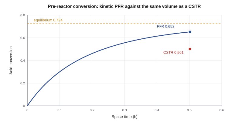
Here \(\tau\) is the space time, the reactor volume divided by the volumetric flow, and \(C_{A0}\) is the inlet concentration of acid, 7.0 kmol per cubic meter. In practice the rate constant is a resin-specific value that depends on temperature through an Arrhenius term and on the catalyst loading. The code fits \(k\) so that the plug flow model gives the design conversion at the design space time, then integrates the profile with a fourth-order Runge-Kutta method, and compares a CSTR of the same volume.
# Three reactor models for the esterification pre-reactor: stoichiometric, equilibrium and kinetic (CSTR and PFR)
import math
K = 4.0        # equilibrium constant (illustrative, nearly independent of temperature)
M = 1.2        # ethanol to acid feed ratio
CA0 = 7.0      # acid concentration in the feed, kmol/m3 (illustrative)
q = 5.7        # volumetric flow, m3/h
V = 2.86       # resin bed volume, m3 (from CHE-345)
def rate_term(X): return (1 - X) * (M - X) - X * X / K
# 1. Stoichiometric reactor: conversion is simply specified
print("stoichiometric model: conversion specified as 0.652 (no information about volume)")
# 2. Equilibrium reactor: solve the quadratic for the extent
a, b, c = 1 - 1 / K, -(1 + M), M
Xeq = (-b - math.sqrt(b * b - 4 * a * c)) / (2 * a)
print(f"equilibrium model: X_eq = {Xeq:.3f}")
# 3a. Kinetic PFR, dX/dtau = k CA0 rate_term(X), integrated with RK4; find k that matches the design conversion
def pfr(k, tau, n=400):
    X, h, prof = 0.0, tau / n, []
    f = lambda X: k * CA0 * rate_term(X)
    for i in range(n):
        k1 = f(X); k2 = f(X + h * k1 / 2); k3 = f(X + h * k2 / 2); k4 = f(X + h * k3)
        X += h * (k1 + 2 * k2 + 2 * k3 + k4) / 6
        if (i + 1) % 80 == 0: prof.append(((i + 1) * h, X))
    return X, prof
tau = V / q
lo, hi = 0.01, 5.0
for _ in range(60):
    k = 0.5 * (lo + hi)
    lo, hi = (k, hi) if pfr(k, tau)[0] < 0.652 else (lo, k)
X, prof = pfr(k, tau)
print(f"space time {tau:.3f} h; fitted rate constant k = {k:.4f} m3/(kmol h) gives X = {X:.3f} in the PFR")
for t, x in prof: print(f"   tau = {t:.3f} h   X = {x:.3f}")
# 3b. Same volume as a CSTR: X = k CA0 tau rate_term(X), solved by Newton
g = lambda X: X - k * CA0 * tau * rate_term(X)
dg = lambda X: 1 - k * CA0 * tau * (-(M - X) - (1 - X) - 2 * X / K)
Xc = 0.5
for _ in range(30): Xc -= g(Xc) / dg(Xc)
print(f"CSTR of the same volume: X = {Xc:.3f}")
# volume a CSTR would need for 0.652
Vc = 0.652 / (k * CA0 * rate_term(0.652)) * q
print(f"CSTR volume needed for X = 0.652: {Vc:.2f} m3 ({Vc / V:.1f} times the PFR)")stoichiometric model: conversion specified as 0.652 (no information about volume) equilibrium model: X_eq = 0.724 space time 0.502 h; fitted rate constant k = 0.4998 m3/(kmol h) gives X = 0.652 in the PFR tau = 0.100 h X = 0.301 tau = 0.201 h X = 0.462 tau = 0.301 h X = 0.557 tau = 0.401 h X = 0.615 tau = 0.502 h X = 0.652 CSTR of the same volume: X = 0.501 CSTR volume needed for X = 0.652: 12.58 m3 (4.4 times the PFR)
The profile shows the typical shape of a reversible reaction. Conversion rises quickly at first, reaching 30 % in the first fifth of the bed, then more slowly as the reverse reaction catches up. By the outlet the net rate has fallen to less than a tenth of its initial value, because the forward and reverse rates are nearly in balance. A CSTR of the same 2.86 cubic meters would reach only 50.1 %, because it operates entirely at the outlet composition, where the rate is lowest. To reach the same 65.2 %, a CSTR would need 12.6 cubic meters, 4.4 times the plug flow volume. This is why fixed beds are preferred for this duty.
Worked problem
Space time and volume
A plug flow reactor processes 5.7 cubic meters per hour of feed with a space time of 0.502 h. What is its volume? If throughput increases by 10 % with the same reactor, what is the new space time?
Show solution
- Volume \(V = \tau q = 0.502 \times 5.7 = 2.86\) cubic meters.
- New flow \(q = 1.10 \times 5.7 = 6.27\) cubic meters per hour.
- New space time \(\tau = 2.86 / 6.27 = 0.456\) h.
- From the profile, conversion at 0.456 h is between 0.615 and 0.652, about 0.637.
Answer: 2.86 cubic meters; the space time falls to 0.456 h and the conversion to about 63.7 %, a drop the kinetic model predicts and the stoichiometric model could not.
Energy balance and temperature
Esterification is mildly exothermic, with a heat of reaction of a few kilojoules per mole, so the pre-reactor runs close to adiabatic with a small temperature rise. The kinetic model includes the energy balance, so it predicts the temperature profile along the bed as well as the conversion. For strongly exothermic reactions, the energy balance dominates: the reactor may need cooling, and the model may show a hot spot. A reactor model that is solved isothermally when the real reactor is adiabatic, or the reverse, is a common error, and Theo checks that the model's thermal mode matches the plant: adiabatic for R-101.
Ion-exchange resins have a maximum operating temperature, often stated by the manufacturer as somewhere above 100 °C for the most stable sulfonic acid resins, and the model should be used to confirm that no part of the bed approaches it in any operating case. Theo adds a check to every case study that reports the maximum bed temperature alongside the conversion.
Catalyst deactivation and parameter uncertainty
Every kinetic parameter carries uncertainty from the data it was fitted to. Malik's demonstration runs covered feed temperatures from 70 to 90 °C and molar ratios from 1.0 to 1.5, and the fitted activation energy has a confidence interval of about ten percent either way. Theo records those ranges in the model log beside the parameters. Results for feed temperatures or ratios outside them are labeled as extrapolations. Where a decision depends heavily on a kinetic result, he runs the model at the ends of the confidence interval as well as at the best estimate, so that the decision can be seen to hold, or not, across the plausible range.
Resin catalysts lose activity over months of service, by fouling and by loss of acid sites. The kinetic model handles this by multiplying the rate constant by an activity factor that falls from one. Malik's demonstration data suggest that activity fell by roughly a fifth over the first year, then stabilized. Theo runs the model at an activity of 0.8 and finds that the outlet conversion falls to about 61.5 %. The reactive column absorbs the difference, because it continues the reaction, but its reboiler duty rises slightly. That result goes into the operating envelope in the design basis.
| Model | Needs | Predicts | Typical use |
|---|---|---|---|
| Yield | Product yields | Balances only | Complex chemistry from pilot data |
| Stoichiometric | Reactions and conversions | Composition, duty | First heat and material balance |
| Equilibrium | Reactions and equilibrium constants | Limit of conversion | Fast reactions; checking other models |
| Gibbs | Species list only | Equilibrium of many species | Combustion, reforming |
| CSTR | Rate equations, volume | Conversion, temperature | Stirred tanks |
| PFR | Rate equations, volume, geometry | Profiles along the reactor | Tubular and packed beds |
Common mistakes
MistakeSpecifying a conversion above equilibrium in a stoichiometric reactor.
InsteadCheck every specified conversion against an equilibrium calculation.
MistakeUsing a kinetic model outside the temperature range of its data.
InsteadRecord the range of the fitted kinetics and flag results outside it.
MistakeModeling an adiabatic bed as isothermal.
InsteadMatch the thermal mode to the plant.
MistakeForgetting catalyst deactivation in the operating envelope.
InsteadRun cases at reduced activity.
Summary and key terms
- Yield and stoichiometric reactors close balances from specified results; they do not predict conversion.
- Equilibrium reactors give the limit of conversion; a Gibbs reactor needs no reaction list.
- Kinetic CSTR and PFR models integrate rate equations and predict the effect of throughput, temperature and catalyst activity.
- For the pre-reactor, a PFR reaches 65.2 %, close to the 72.4 % equilibrium; a CSTR of equal volume reaches only 50.1 %.
- The reactor energy balance and thermal mode must match the real equipment.
- Stoichiometric reactor
- A model that calculates outlet composition from specified conversions or extents.
- Gibbs reactor
- An equilibrium model that minimizes total Gibbs energy subject to element balances.
- CSTR
- An ideal perfectly mixed continuous reactor.
- PFR
- An ideal reactor with no mixing in the direction of flow.
- Space time
- Reactor volume divided by inlet volumetric flow.
- Activity factor
- A multiplier on the rate constant representing catalyst deactivation.
Practice problems
Work each problem on paper first, then reveal the answer to check.
Why is a fixed-conversion reactor called a statement of hope?
Show answer
It cannot predict how conversion changes with operating conditions.
What is the equilibrium conversion of the pre-reactor feed?
Show answer
About 72.4 %.
Why does a CSTR need more volume than a PFR for the same conversion?
Show answer
It operates at the outlet composition, where the rate is lowest.
How much larger is the CSTR volume for 65.2 %?
Show answer
About 4.4 times, 12.6 cubic meters against 2.86.
What happens to space time if flow rises 10 %?
Show answer
It falls from 0.502 to 0.456 h.
How is catalyst deactivation represented?
Show answer
By an activity factor multiplying the rate constant.
Lesson quiz · 5 questions
Score 60% or more to complete this lesson.
Create a free account to save your progress, take quizzes and earn a certificate.