
CHE-460 · Lesson 1 of 12 · 24 min
What process simulation is and how a model is built
In December, Kingfisher Bioenergy's board approved option D for the ethyl acetate line at Cedar Rapids: the base process with mechanical vapor recompression on the ester column and a long-term contract for acetic acid. The design that Theo, now an engineer-in-training, helped to sanction in CHE-446 was built on spreadsheets, shortcut methods and hand-checked balances. Detailed engineering needs more. The contractor's process engineers will size every vessel, nozzle and relief valve from a rigorous model, and the operators will learn the new controls on a training simulator built from that same model. Ingrid Solheim, Theo's mentor, asks him to own the owner's copy of the process model: to build it, check it against the contractor's, and use it to answer the questions the project will keep asking for the next three years.
This course follows that work. Process simulation is the use of a mathematical model of a process, solved on a computer, to predict how the process will behave. A simulator does not know chemistry or physics by itself. It holds libraries of property data and thermodynamic models, a set of unit operation models that apply mass, energy and equilibrium relations to each piece of equipment, and numerical methods that solve all of those equations together. The engineer chooses the components, the property methods, the units and how they connect, and the values that pin the problem down. The answers are only as good as those choices.
What simulators are used for
Steady-state simulation predicts the flows, compositions, temperatures, pressures and duties of a process running at constant conditions. It is the workhorse of design: it produces the heat and material balance on which equipment is sized, it compares process options, and it supports debottlenecking and troubleshooting of existing plants. Dynamic simulation adds time. It follows the inventories in vessels, the response of controllers and the behavior of the plant during start-up, shutdown, upsets and emergencies. It is used to design control systems, check relief scenarios and train operators.
Commercial simulators dominate industrial practice. Aspen Plus and Aspen HYSYS, gPROMS, Pro/II and UniSim are widely used, and each has a large library of components, property methods and unit models. Open tools also exist. DWSIM is an open-source process simulator; COCO with the ChemSep column model is free to use; and general-purpose languages such as Python, with libraries for equation solving and thermodynamics, let engineers write small models themselves. This course does not teach the buttons of any one product. It teaches what every simulator is doing underneath, so that an engineer can use any of them critically. The code in each lesson is written in plain Python with no special libraries, so every number can be traced.
The modeling workflow
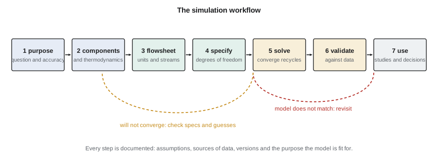
Ingrid gives Theo a list that every good simulation follows. First, state the purpose. A model built to size a column is not automatically fit to predict trace impurities in the product, and a model for an operator training simulator needs dynamics that a design model does not. The purpose sets the accuracy needed and the level of detail. Second, choose the components and the thermodynamic method, the single most important decision in the model, covered in lesson 3. Third, draw the flowsheet: units, streams, and how they connect. Fourth, specify enough variables to fix the problem, which is a question of degrees of freedom. Fifth, solve it, which for any plant with recycles means converging tear streams, covered in lesson 7. Sixth, validate the model against plant data, pilot data or trusted references. Seventh, use it.
The loops back are where the work lies. A model that will not converge usually has a specification that is impossible or inconsistent, poor initial guesses, or a thermodynamic method that predicts an extra liquid phase nobody expected. A model that converges but does not match data may have the wrong property method, the wrong efficiency assumed for a column, or simply a mistake in a feed. Ingrid's rule is that a converged model is not a correct model. Convergence means only that the equations are satisfied; whether they are the right equations is a separate question.
Degrees of freedom
A unit model is a set of equations in a set of variables. The number of degrees of freedom is the number of variables minus the number of independent equations. The engineer must specify exactly that many variables; the simulator calculates the rest. Specify too few and the problem has infinitely many solutions; too many and it has none, or the simulator rejects the input.
Consider a flash drum: a feed enters, a vapor and a liquid leave in equilibrium, and heat may be added. With \(c\) components, the variables are the flow, composition, temperature and pressure of each stream, plus the heat duty. The equations are a material balance for each component, one energy balance, an equilibrium relation for each component, the requirement that vapor and liquid leave at the same temperature and pressure, and the requirement that the mole fractions in each stream add to one. Counting carefully shows that once the feed is completely known, two more specifications are needed. Temperature and pressure is the most common pair, but pressure and heat duty, or pressure and vapor fraction, work equally well. Temperature and vapor fraction together also fix the drum, although the simulator must then search for the pressure.
# Degrees of freedom for a flash drum and for a small flowsheet (counting variables and equations)
def flash_dof(nc):
    # streams: feed, vapor, liquid -> each has nc mole fractions... count with flows
    # variables: F, z(nc), TF, PF ; V, y(nc), T, P ; L, x(nc) ; Q
    variables = (nc + 3) + (nc + 3) + (nc + 1) + 1
    # equations: nc component balances, 1 energy balance, nc equilibrium (y = K x),
    # T and P equal in V and L (already shared), sum y = 1, sum x = 1, sum z = 1
    equations = nc + 1 + nc + 3
    return variables, equations, variables - equations
for nc in (2, 3, 4):
    v, e, d = flash_dof(nc)
    print(f"flash drum, {nc} components: {v} variables, {e} equations, {d} specifications needed")
print()
# Feed fully known (nc + 2 specs); the rest must be chosen from T, P, Q, V/F
nc = 3
v, e, d = flash_dof(nc)
feed_specs = nc + 2   # flow, nc-1 fractions, T, P
print(f"after the feed is specified: {d - feed_specs} more specifications (for example T and P)")
print()
# Sequential-modular vs equation-oriented size of the problem
units = {"mixer": 1, "pre-reactor": 1, "reactive column": 25, "decanter": 1, "ester column": 30, "stripper": 15}
nc = 4
eqs = 0
for u, stages in units.items():
    per_stage = 2 * nc + 3   # MESH: nc material + nc equilibrium + 2 summations + 1 enthalpy
    eqs += stages * per_stage
    print(f"{u:16s} {stages:3d} stage(s) -> {stages * per_stage:4d} equations")
print(f"equation-oriented model of the line: about {eqs} equations solved together")flash drum, 2 components: 14 variables, 8 equations, 6 specifications needed flash drum, 3 components: 17 variables, 10 equations, 7 specifications needed flash drum, 4 components: 20 variables, 12 equations, 8 specifications needed after the feed is specified: 2 more specifications (for example T and P) mixer 1 stage(s) -> 11 equations pre-reactor 1 stage(s) -> 11 equations reactive column 25 stage(s) -> 275 equations decanter 1 stage(s) -> 11 equations ester column 30 stage(s) -> 330 equations stripper 15 stage(s) -> 165 equations equation-oriented model of the line: about 803 equations solved together
The same counting works for a whole flowsheet. Each unit adds its own degrees of freedom; each connection removes some, because the outlet of one unit is the inlet of the next. In practice the simulator's input forms are laid out so that the user fills in exactly the right number of values for each unit. Problems arise when the engineer wants to specify something the form does not ask for, such as a product purity instead of a reflux ratio. Then a design specification, covered in lesson 8, swaps one variable for another without changing the count.
Worked problem
Degrees of freedom for a mixer
Two streams of the same three components mix adiabatically in a pipe tee. Both inlets are fully specified. How many more specifications does the mixer need?
Show solution
- Each stream has \(c + 2 = 5\) independent variables: flow, two independent mole fractions, temperature and pressure.
- There are 15 variables in three streams; the 10 for the inlets are given, leaving 5 for the outlet.
- The equations are 3 component balances and 1 energy balance: 4 equations.
- \(5 - 4 = 1\): one more specification is needed, usually the outlet pressure.
Answer: One: the outlet pressure, because the balances cannot set it. Simulators often default it to the lowest inlet pressure.
Two ways to solve a flowsheet
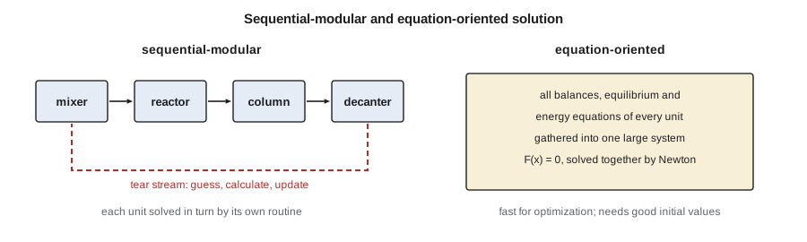
Simulators solve a flowsheet in one of two ways. In the sequential-modular approach, each unit model is a self-contained routine that takes its inlet streams and parameters and calculates its outlets. The simulator calls the units in order, passing streams along. This is intuitive and robust for each unit, because each routine can use a method tuned to its own equations. Its weakness is recycle. When a stream from a later unit returns to an earlier one, the simulator does not know that stream when it starts. It must guess it, calculate round the loop, compare the result with the guess, and repeat until they agree. The guessed stream is called a tear stream. Aspen Plus, HYSYS, DWSIM and most teaching simulators work this way for steady state.
In the equation-oriented approach, all the equations of all the units are gathered into one large system and solved simultaneously, usually by a Newton method. There are no tear streams, because recycles are simply more equations. Specifications can be placed on any variable, and optimization is natural, because an optimizer can change all variables at once. The cost is that the system is large, often tens of thousands of equations for a full plant, and Newton's method needs good starting values. gPROMS works this way, and several commercial simulators offer an equation-oriented mode for optimization and real-time applications. The code above estimates that a rigorous model of the ester line alone has about 800 equations, before counting the energy and pressure relations of pumps, exchangers and controllers.
Accuracy, purpose and the limits of models
Every model is an approximation. Thermodynamic models fit data over a range and extrapolate poorly outside it. Equilibrium stage models assume each tray reaches equilibrium, which none does, and correct for it with an efficiency the user must supply. Kinetic models fitted in a laboratory may not hold at plant scale if mixing or heat removal differs. A good engineer knows where the model is strong and where it is weak, and reports results with that in mind. A reboiler duty from a well-validated model may be trusted to within a few percent; a trace impurity concentration in the product, which depends on activity coefficients at infinite dilution, may be uncertain by a factor of two or more.
Ingrid makes the point with the ester line. The design basis requires ethyl acetate of at least 99.7 % purity, with limits on ethanol, water and acetic acid. The model predicts the main purity well, because it depends on the large, well-measured volatility between the ester and the light azeotrope. It predicts the residual acetic acid less well, because the acid dimerizes in the vapor and its interaction with ester is poorly characterized. Theo writes both facts into the model's documentation, so that whoever uses the model later knows which answers to lean on.
| Question | Steady state? | Dynamic? | Typical detail |
|---|---|---|---|
| Size equipment and utilities | Yes | No | Rigorous units, validated thermodynamics |
| Compare process options | Yes | No | Shortcut models often enough |
| Design control loops | Starting point | Yes | Holdups, valves, controllers |
| Size relief devices for upsets | Sometimes | Yes | Vessel volumes, heat input, time |
| Train operators | No | Yes | Full plant with operator interface |
| Monitor a running plant | Yes, tuned to data | Sometimes | Reconciled measurements |
Documenting and controlling the model
A process model becomes an engineering record. The design basis memorandum from CHE-446 names it as the source of the heat and material balance, which feeds the equipment data sheets, which feed the purchase orders. When a number changes in the model, it changes downstream. Kingfisher Bioenergy therefore keeps the model under the same change control as drawings: each issued version has a number, a date, a list of changes and the name of the engineer who checked it. The professional engineer who seals the process design, a licensed PE under the Iowa Engineering and Land Surveying Examining Board, relies on that record. A simulation result is not a calculation that can be sealed on its own; the engineer is responsible for the inputs, the method choices and the checks behind it.
Good documentation records the purpose; the component list and its data sources; the property method with any regressed parameters and the data they came from; each unit model with its specifications and efficiencies; the convergence settings; and the validation, including where the model disagrees with data and by how much. It also records what the model is not fit for. Theo starts a model log on the first day, and writes a line for every change. It is dull, and it saves weeks when a contractor asks why the owner's model gives a different reboiler duty from theirs.
Checking the results of any simulation
Ingrid's checklist for any simulator output is short. Do the overall material and energy balances close? Are the temperatures and pressures physically sensible, with no streams below their freezing point or above their critical point by accident? Are the phases what you expect, or has the property method found a second liquid phase in the column? Do the duties have the right sign and order of magnitude? Does a shortcut hand calculation give a result within the expected range? A simulator will happily report a converged column with the feed on the wrong tray, a heat exchanger with a temperature cross, or a reactor that produces more product than the feed can make if a specification is wrong. The engineer, not the software, catches those.
Common mistakes
MistakeTreating a converged model as a correct one.
InsteadConvergence means the equations are satisfied; validation shows they are the right equations.
MistakeSpecifying variables until the simulator stops complaining.
InsteadCount degrees of freedom and choose specifications that the plant can actually set.
MistakeUsing one model for every purpose.
InsteadState the purpose first; detail and accuracy follow from it.
MistakeChanging the model without recording why.
InsteadKeep the model under change control like any other engineering record.
Summary and key terms
- Process simulation solves a mathematical model of the process to predict steady or dynamic behavior.
- The engineer chooses components, property methods, units, connections and specifications; the simulator does the arithmetic.
- Degrees of freedom equal variables minus equations; a flash drum with a known feed needs two more specifications.
- Sequential-modular simulators solve units in turn and converge recycles with tear streams; equation-oriented simulators solve everything together.
- A model is fit for a stated purpose, must be validated, and must be documented and controlled as an engineering record.
- Process simulation
- Solving a mathematical model of a process on a computer to predict its behavior.
- Degrees of freedom
- The number of variables that must be specified for a model to have a unique solution.
- Sequential-modular
- A solution strategy that calculates each unit in turn and converges recycles by iteration.
- Equation-oriented
- A solution strategy that solves all the equations of a flowsheet together.
- Tear stream
- A recycle stream that is guessed and then updated until the calculated value matches the guess.
- Validation
- Checking that a model reproduces measured data within an accepted tolerance.
Practice problems
Work each problem on paper first, then reveal the answer to check.
How many specifications does a flash drum need once its feed is known?
Show answer
Two, for example temperature and pressure.
Why does a sequential-modular simulator need tear streams?
Show answer
A recycle stream is unknown when the calculation reaches the first unit, so it must be guessed and updated.
Name one advantage of an equation-oriented solver.
Show answer
Specifications and optimization variables can be placed on any variable, and recycles need no tearing.
Why is a trace impurity prediction less certain than a main purity?
Show answer
It depends on activity coefficients at infinite dilution, which are poorly known.
What should a model log record?
Show answer
Purpose, components and data sources, property methods, unit specifications, convergence settings, validation and every change.
Give two quick checks on any simulation result.
Show answer
Overall balances close; temperatures, pressures, phases and duties are physically sensible.
Lesson quiz · 5 questions
Score 60% or more to complete this lesson.
Create a free account to save your progress, take quizzes and earn a certificate.