
CHE-460 · Lesson 10 of 12 · 21 min
Dynamic simulation
Everything so far has been steady state: the plant running at constant conditions, with every accumulation term set to zero. Real plants are never quite steady. Feeds change, cooling water warms through the day, catalysts age, and operators start up, shut down and respond to upsets. Wren's operations team will run the new line, and she wants answers that steady-state models cannot give. How fast does the reflux drum level move when boil-up changes? How long do operators have if cooling water fails? Will the control scheme designed in CHE-374 actually hold the purity through a feed swing? These are questions for dynamic simulation.
From steady state to dynamics
A dynamic model restores the accumulation terms. Each vessel, tray and pipe with significant holdup gets differential equations for its mass, component and energy inventories. Flows are no longer fixed numbers but depend on pressure differences and valve openings. Controllers, with their tuning, measure and act. The model becomes a large system of differential and algebraic equations, integrated forward in time.
A dynamic model needs information a steady-state model does not. Vessel dimensions set the holdups. Valve sizes and characteristics set how flow responds to opening. Pump curves, line resistances and elevations set pressures. Controllers need their algorithms, tuning and ranges. Tray hydraulics determine how liquid holdup changes with flow. In practice, the steady-state model is the starting point: it is converted to dynamic mode by adding this equipment data, and it starts the dynamic run from the converged steady state. Aspen HYSYS and Aspen Plus Dynamics, gPROMS, UniSim and DWSIM all offer dynamic modes, and specialized operator training simulators are built on similar engines.
Numerical integration
The differential equations are integrated by numerical methods. The simplest, the explicit Euler method, steps forward using the current derivative. It is easy and often inaccurate unless the step is small. The fourth-order Runge-Kutta method, RK4, evaluates the derivative four times per step and is far more accurate for the same step size. Process models raise a further difficulty, stiffness: some parts of the model, such as pressure in a small gas space or the composition on a tray with little holdup, respond in seconds, while others, such as a large tank level, take hours. Explicit methods must use a step small enough for the fastest part, which can make them very slow. Implicit methods, such as backward differentiation formulas, remain stable with large steps and are the standard in dynamic simulators.
A reflux drum under level control
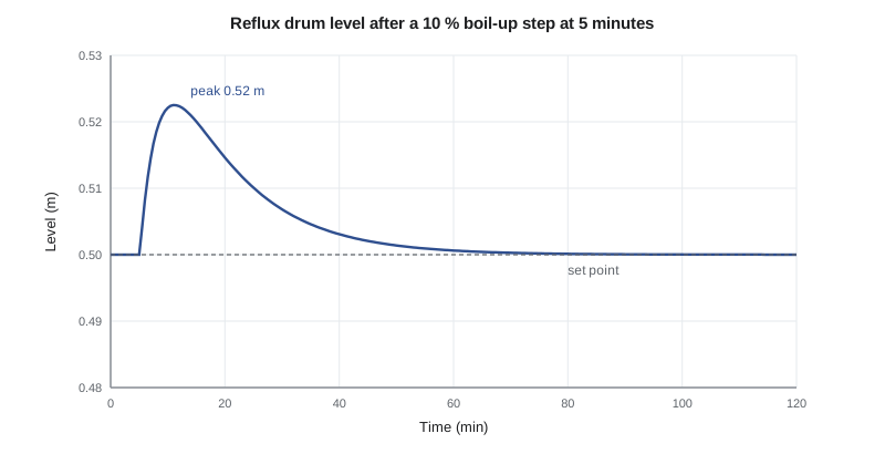
The first part of the code simulates the ester column reflux drum. Vapor from the column condenses into the drum; reflux returns to the column in a fixed ratio to the condensed flow, as in the CHE-374 control scheme; and the distillate valve is manipulated by a PI level controller with gain 1.67 and integral time 16 minutes, the tuning chosen in that course. At 5 minutes the boil-up steps up by 10 %, as it might when steam pressure rises. The model integrates the drum holdup and the controller's integral term together with RK4, using a step of three seconds.
# Dynamic simulation: reflux drum level under PI control after a boil-up step, and pressure rise on loss of cooling
# Part 1: drum holdup (kmol) with RK4; distillate valve on PI level control; time in minutes
A_drum = 6.0                 # kmol of liquid per meter of level (illustrative 1.2 m diameter horizontal drum, linearized)
Kc, Ti = 1.67, 16.0          # controller tuning from CHE-374 (% output per % level, minutes)
span_level, span_flow = 1.0, 80.0    # m for 0-100 % level; kmol/h for 0-100 % valve
V0, R = 89.4, 1.34           # boil-up (kmol/h) and reflux ratio, design point
D0 = V0 / (R + 1)
def run(step_frac, t_end=120.0, dt=0.05):
    h, integ, t = 0.5, 0.0, 0.0              # level m, integral of error, min
    sp = 0.5; out, peak, n = [], 0.5, 0
    def deriv(h, integ, t):
        V = V0 * (1 + (step_frac if t >= 5.0 else 0.0))
        Lr = R * D0 * (V / V0)                 # reflux set in ratio to the condensed vapor
        e = (h - sp) / span_level * 100        # % level error (direct acting: high level opens the valve)
        u = 100 * D0 / span_flow + Kc * (e + integ / Ti)
        u = max(0.0, min(100.0, u))
        D = u / 100 * span_flow
        dh = (V - Lr - D) / 60 / A_drum        # m/min
        return dh, e
    while t < t_end:
        k1 = deriv(h, integ, t); k2 = deriv(h + dt * k1[0] / 2, integ + dt * k1[1] / 2, t + dt / 2)
        k3 = deriv(h + dt * k2[0] / 2, integ + dt * k2[1] / 2, t + dt / 2); k4 = deriv(h + dt * k3[0], integ + dt * k3[1], t + dt)
        h += dt * (k1[0] + 2 * k2[0] + 2 * k3[0] + k4[0]) / 6
        integ += dt * (k1[1] + 2 * k2[1] + 2 * k3[1] + k4[1]) / 6
        t += dt; n += 1; peak = max(peak, h)
        if n % int(round(10 / dt)) == 0: out.append((round(t), h))
    return out, peak
out, peak = run(0.10)
print("boil-up +10 % at t = 5 min; reflux drum level (m), set point 0.50 m")
for t, h in out: print(f"   t = {t:4d} min   level {h:.3f} m")
print(f"peak level {peak:.3f} m ({(peak - 0.5) / span_level * 100:.1f} % of span above set point)")
print()
# Part 2: loss of cooling water; vapor keeps coming from the reboiler; gas space pressurizes (ideal gas)
Rg, T = 8.314, 350.0         # kJ/(kmol K), K
Vgas = 14.0                  # m3 of vapor space in the column top, overhead line and drum (illustrative)
P, t, dt = 101.3, 0.0, 0.5   # kPa, s
Vin = V0 / 3600              # kmol/s of vapor still arriving
Pset = 350.0                 # relief valve set pressure, kPa absolute (illustrative)
while P < Pset:
    P += Rg * T / Vgas * Vin * dt; t += dt
print(f"with no condensation the top pressure reaches the {Pset:.0f} kPa relief set point in about {t:.0f} s ({t / 60:.1f} min)")
print("a high-pressure trip of the reboiler steam at 250 kPa acts first if it works:")
P, t = 101.3, 0.0
while P < 250.0: P += Rg * T / Vgas * Vin * dt; t += dt
print(f" trip reached after about {t:.0f} s, about {Pset - 250:.0f} kPa below the relief set point")boil-up +10 % at t = 5 min; reflux drum level (m), set point 0.50 m t = 10 min level 0.522 m t = 20 min level 0.515 m t = 30 min level 0.507 m t = 40 min level 0.503 m t = 50 min level 0.501 m t = 60 min level 0.501 m t = 70 min level 0.500 m t = 80 min level 0.500 m t = 90 min level 0.500 m t = 100 min level 0.500 m t = 110 min level 0.500 m t = 120 min level 0.500 m peak level 0.522 m (2.2 % of span above set point) with no condensation the top pressure reaches the 350 kPa relief set point in about 48 s (0.8 min) a high-pressure trip of the reboiler steam at 250 kPa acts first if it works: trip reached after about 29 s, about 100 kPa below the relief set point
The level rises to a peak of 0.522 m, 2.2 % of span above set point, then returns smoothly to 0.500 m over about an hour. That is the behavior wanted from averaging level control: the drum absorbs the disturbance, and the distillate flow changes gradually rather than passing the full step to the stripper and the decanter. If Theo raises the gain, the peak falls but the distillate swings more; the dynamic model lets the team see that trade-off before the plant exists.
Worked problem
Drum level rate of rise
A drum holds 6.0 kmol of liquid per meter of level. If inflow exceeds outflow by 5.6 kmol/h and the controller has not yet acted, how fast does the level rise?
Show solution
- Rate of rise = imbalance / holdup per meter.
- \(5.6 / 6.0 = 0.93\) m per hour.
- Per minute: \(0.93 / 60 = 0.016\) m per minute.
- In 5 minutes, with no control action, the level would rise about 0.08 m.
Answer: About 0.016 m per minute. The controller acts well before the level rises that far, which is why the peak is only 0.022 m.
Upsets and relief
Dynamic models are increasingly used to study abnormal situations, including those that set relief requirements. The second part of the code considers total loss of cooling water to the ester column condenser. The reboiler continues to boil up vapor, which no longer condenses, so the vapor space of the column top, overhead line and drum pressurizes. A simple ideal-gas model with 14 cubic meters of vapor space and the full design boil-up reaches the relief set pressure of 350 kPa absolute in about 48 seconds. A high-pressure trip on the reboiler steam, set at 250 kPa, is reached in about 29 seconds.
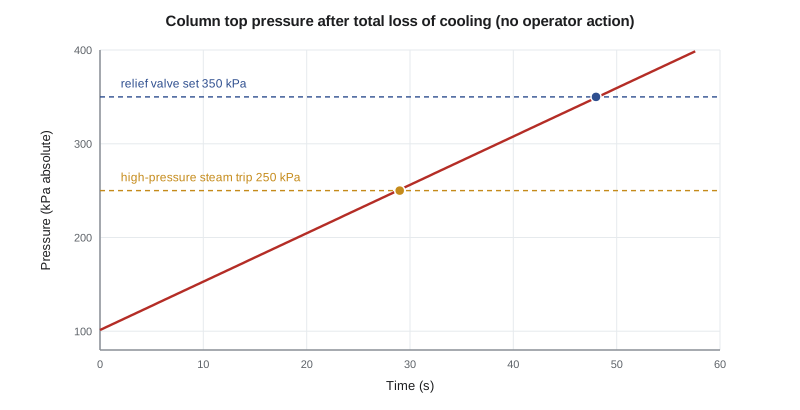
Ingrid points out what this simple model leaves out, and in which direction each omission errs. As the pressure rises, the boiling point at the bottom rises, the temperature difference across the reboiler falls, and boil-up drops: the real rise is slower. Some vapor condenses on cold metal and in the liquid on the trays at first: slower again. But the condenser may not lose all its cooling at once, and the vapor may be hotter than assumed. The simple model is conservative in most respects, and it shows two things clearly: operators have seconds, not minutes, so the protection must be automatic; and the steam trip is a real layer of protection, acting before relief. Relief sizing itself follows recognized practice, such as API Standard 521 and the requirements under OSHA's Process Safety Management standard, 29 CFR 1910.119, together with EPA's Risk Management Program rule where a listed chemical exceeds its threshold quantity, and for complex cases dynamic simulation of the relief scenario is accepted as a basis for the relief load. That work belongs to the contractor's relief specialists and is checked in the process hazard analysis.
Testing control strategies
The most common use of dynamic simulation in design is to test the control strategy. Theo builds the 17 loops from CHE-374 into the dynamic model of the ester column and decanter, and runs a set of disturbances: feed composition swings of ±5 %, a 10 % throughput change, a drop in cooling water temperature, and a step in steam pressure. For each he checks that product purity stays within specification and that no level or pressure reaches an alarm limit. Two findings come back to the control design. The tray 18 temperature controller, tuned for the original steam reboiler, is too aggressive with the vapor recompression system, whose compressor responds more slowly than a steam valve; it needs detuning. And a feed composition swing of 5 % takes about 40 minutes to show at the bottoms analyzer, confirming that the temperature control, not the analyzer, must carry the fast correction.
| Aspect | Steady-state model | Dynamic model |
|---|---|---|
| Accumulation | Zero | Holdups in vessels and trays |
| Flows | Specified or calculated from balances | From pressure differences and valve openings |
| Controllers | Represented by specifications | Algorithms, tuning and ranges |
| Equipment data needed | Few dimensions | Volumes, valves, pumps, hydraulics |
| Solution | Algebraic equations | Differential-algebraic equations integrated in time |
| Typical uses | Design balances, optimization | Control design, upsets, start-up, training |
Operator training simulators
An operator training simulator connects a dynamic plant model to a copy of the plant's control system screens, so that operators can practice normal and emergency operations without risk. For a new line, it also lets operators learn the plant before it starts, and lets engineers check the control system configuration and operating procedures. Wren plans to have her operators train on a simulator of the new line for several weeks before commissioning, including the loss of cooling scenario and a recompressor trip. The model for the simulator comes from the same validated process model, tuned further when the plant runs.
Common mistakes
MistakeRunning a dynamic model without real equipment data.
InsteadEnter vessel sizes, valve characteristics and pump curves from data sheets.
MistakeUsing an explicit integrator on a stiff model.
InsteadUse the simulator's implicit methods, or a step small enough for the fastest dynamics.
MistakeTreating a simple upset model as the relief design.
InsteadUse it to understand timing; relief sizing follows recognized practice and the hazard analysis.
MistakeTesting only one disturbance.
InsteadTest a set of realistic disturbances against purity and alarm limits.
Summary and key terms
- Dynamic models restore accumulation terms and need holdups, valves, pumps and controllers.
- Integration uses Runge-Kutta or, for stiff models, implicit methods.
- Averaging level control holds the reflux drum to a 2.2 % peak after a 10 % boil-up step while smoothing distillate flow.
- Loss of cooling pressurizes the column top in under a minute; automatic protection is essential.
- Dynamic models test control strategies and form the basis of operator training simulators.
- Dynamic simulation
- Simulation that follows how a process changes with time.
- Holdup
- The inventory of material in a vessel, tray or pipe.
- Stiffness
- The presence of very fast and very slow dynamics in the same model.
- RK4
- The fourth-order Runge-Kutta integration method.
- Implicit method
- An integration method that solves for the new state using its own derivative, stable at large steps.
- Operator training simulator
- A dynamic plant model connected to control screens for training.
Practice problems
Work each problem on paper first, then reveal the answer to check.
What information does a dynamic model need that a steady-state one does not?
Show answer
Holdups, valve characteristics, pump curves, hydraulics and controller tuning.
What peak did the drum level reach after the step?
Show answer
0.522 m, 2.2 % of span above set point.
Why are implicit integrators used in dynamic simulators?
Show answer
Process models are stiff, and implicit methods stay stable with large steps.
How long until relief pressure in the simple loss-of-cooling model?
Show answer
About 48 seconds.
Name one way the simple pressure model is conservative.
Show answer
It ignores the fall in boil-up as pressure rises.
What did dynamic testing reveal about the tray 18 controller?
Show answer
It was too aggressive with the slower vapor recompression system.
Lesson quiz · 5 questions
Score 60% or more to complete this lesson.
Create a free account to save your progress, take quizzes and earn a certificate.