Partial molar properties and mixing

Dev Raman in the quality control lab has a puzzle for Theo. A technician blended 50 L of anhydrous ethanol with 50 L of water to make a calibration standard and measured the volume of the result: about 97 L, not 100. Nothing leaked. The missing volume is a property of the mixture, and it is the clearest everyday sign that a solution is not just a sum of its parts. The tools for describing it are partial molar properties, which also turn out to be the bridge between the chemical potential of lesson 1 and the measurable properties of real mixtures.

Mixture properties are not simply additive

For an ideal mixture, a total property such as volume would be the sum of the pure-component contributions: \(nV = \sum n_i V_i\). Ethanol and water break that rule because the molecules interact differently with each other than with their own kind. Hydrogen bonds between ethanol and water, and the way small water molecules fit into the spaces around larger ethanol molecules, pack the mixture more tightly than either pure liquid. The same is true, to different degrees, of enthalpy, entropy and Gibbs energy. Engineers handle all of these with one idea.

Partial molar properties

For any extensive property \(M\) (volume, enthalpy, entropy, Gibbs energy), the partial molar property of species \(i\) is

It is the change in the total property when a small amount of \(i\) is added to a large amount of mixture, per mole added, with temperature, pressure and the amounts of everything else held constant. The total property of the mixture is then exactly the mole-weighted sum of the partial properties:

This summability relation looks like the ideal-mixture rule, but with partial molar properties in place of pure-component ones. The chemical potential of lesson 1 is simply the partial molar Gibbs energy: \(\mu_i = \bar{G}_i\). Everything learned about partial molar properties therefore applies to the chemical potential too.

The Gibbs-Duhem equation

Partial molar properties in a mixture are not independent. Differentiating the summability relation and comparing it with the general expression for \(d(nM)\) gives, at constant temperature and pressure,

This is the Gibbs-Duhem equation. For a binary it says that if the partial molar volume of ethanol rises as ethanol is added, the partial molar volume of water must fall, by an amount fixed by the mole fractions. It has two practical uses. First, if one partial property is measured across the whole composition range, the other can be calculated. Second, it gives a consistency test for experimental data: measured activity coefficients that violate the Gibbs-Duhem equation contain errors, a test lesson 6 applies to ethanol-water vapor-liquid data.

Excess and mixing properties

The property change of mixing is the difference between the mixture and the pure components at the same temperature and pressure: \(\Delta M = M - \sum x_i M_i\). For volume, the 3 L shrinkage in Dev's blend is \(n\Delta V\). For an ideal solution, the volume and enthalpy of mixing are zero, but the entropy of mixing is not: \(\Delta S^{\text{id}} = -R\sum x_i\ln x_i\), which is always positive, and so the ideal Gibbs energy of mixing \(\Delta G^{\text{id}} = RT\sum x_i\ln x_i\) is always negative. The excess property measures how far a real solution departs from ideal: \(M^E = M - M^{\text{id}}\). For volume and enthalpy the excess and mixing properties are the same thing; for entropy and Gibbs energy they are not, because the ideal solution already has a nonzero entropy of mixing.

The excess Gibbs energy \(G^E\) is the most important of these. Lesson 6 shows that its partial molar form is \(RT\ln\gamma_i\), the logarithm of the activity coefficient, and lesson 7's models for activity coefficients are all expressions for \(G^E\) as a function of composition. Getting comfortable with excess properties here pays off in every later lesson.

Fitting an excess volume and reading partial molar volumes

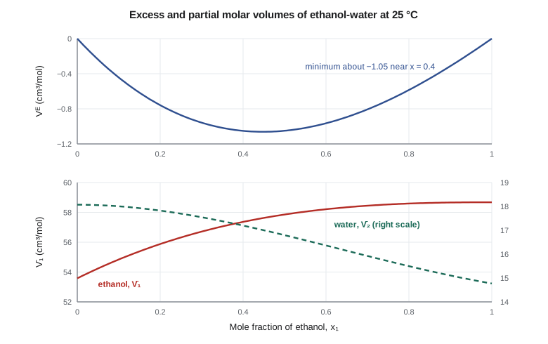
Measured excess volumes of binary liquids are commonly fitted with a Redlich-Kister series, \(V^E = x_1x_2[a_0 + a_1(x_1 - x_2) + \dots]\), which goes to zero at both pure-component ends as it must. For ethanol-water at 25 °C, two terms with \(a_0 = -4.2\) and \(a_1 = 0.9\) cm\(^3\)/mol describe the data well enough for this lesson; the minimum excess volume is about \(-1.05\) cm\(^3\)/mol near \(x_1 = 0.4\). These constants are approximate, rounded from the published density data.

The partial molar volumes come from the tangent-intercept construction. Draw the tangent to the curve of molar volume against \(x_1\) at the composition of interest; its intercepts at \(x_1 = 1\) and \(x_1 = 0\) are \(\bar{V}_1\) and \(\bar{V}_2\). Algebraically, for a binary, \(\bar{V}_1 = V + x_2\,dV/dx_1\) and \(\bar{V}_2 = V - x_1\,dV/dx_1\). The code applies these to the fitted curve.

# Partial molar volumes of ethanol (1) and water (2) at 25 C from a Redlich-Kister fit of excess volume
# Pure molar volumes and fit constants are approximate textbook-scale values.
V1, V2 = 58.68, 18.07          # cm3/mol, pure ethanol and pure water
a0, a1 = -4.20, 0.90           # cm3/mol, VE = x1 x2 [a0 + a1 (x1 - x2)]

def VE(x1):
    x2 = 1 - x1
    return x1 * x2 * (a0 + a1 * (x1 - x2))

def dVE(x1, h=1e-6):
    return (VE(x1 + h) - VE(x1 - h)) / (2 * h)

print(" x1     VE      Vbar1   Vbar2")
for x1 in (0.0, 0.1, 0.2, 0.3, 0.4, 0.5, 0.7, 0.9, 1.0):
    x2 = 1 - x1
    d = dVE(min(max(x1, 1e-6), 1 - 1e-6))
    vb1 = V1 + VE(x1) + x2 * d        # partial molar volume from the tangent-intercept rule
    vb2 = V2 + VE(x1) - x1 * d
    print(f"{x1:4.1f}  {VE(x1):6.3f}  {vb1:6.2f}  {vb2:6.2f}")

# Blending 50 L of ethanol with 50 L of water
n1 = 50000 / V1; n2 = 50000 / V2
x1 = n1 / (n1 + n2)
V = n1 * V1 + n2 * V2 + (n1 + n2) * VE(x1)
print(f"x1 = {x1:.3f}; mixture volume = {V / 1000:.1f} L, shrinkage = {100 - V / 1000:.1f} L")

# Gibbs-Duhem check: x1 dVbar1 + x2 dVbar2 should be zero
x1, h = 0.3, 1e-4
def vbars(x):
    d = dVE(x); return V1 + VE(x) + (1 - x) * d, V2 + VE(x) - x * d
a, b = vbars(x1 - h), vbars(x1 + h)
print(f"Gibbs-Duhem residual at x1 = 0.3: {x1 * (b[0] - a[0]) + (1 - x1) * (b[1] - a[1]):.2e} cm3/mol")

 x1     VE      Vbar1   Vbar2
 0.0  -0.000   53.58   18.07
 0.1  -0.443   54.84   18.00
 0.2  -0.758   55.88   17.82
 0.3  -0.958   56.71   17.55
 0.4  -1.051   57.36   17.20
 0.5  -1.050   57.85   16.80
 0.7  -0.806   58.45   15.92
 0.9  -0.313   58.66   15.11
 1.0  -0.000   58.68   14.77
x1 = 0.235; mixture volume = 97.0 L, shrinkage = 3.0 L
Gibbs-Duhem residual at x1 = 0.3: 7.19e-12 cm3/mol

What the numbers say

The partial molar volume of ethanol falls from 58.68 cm\(^3\)/mol when pure to about 53.6 cm\(^3\)/mol at infinite dilution in water. A few drops of ethanol added to a beaker of water add about 54 cm\(^3\) per mole, not 59. Water, for its part, occupies only about 14.8 cm\(^3\)/mol when it is dilute in ethanol, compared with 18.07 pure. The Gibbs-Duhem check prints a residual near \(10^{-11}\), confirming that partial properties derived consistently from one function of composition automatically satisfy it.

Dev's blend has \(x_1 = 0.235\), and the model gives 97.0 L, a 3.0 L shrinkage. The measured volume was about 97 L, so the fit is serviceable. The practical lessons for the plant are direct. Tank inventories of ethanol-water mixtures cannot be found by adding volumes; they need density and mass. Custody transfer of fuel ethanol is done on corrected volumes or by mass for exactly this reason. And alcohol content is quoted carefully as mass percent, volume percent or proof, which are not interchangeable.

Heat of mixing

The enthalpy of mixing of ethanol and water is also nonzero. Near room temperature, mixing is exothermic, releasing up to about 0.8 kJ per mole of mixture near \(x_1 = 0.2\) to 0.3; at higher temperatures the sign changes over part of the range. A plant blending large flows of hydrous ethanol and water will see a temperature rise of a few degrees, which matters for density corrections and vapor losses from tanks. Excess enthalpy is also tied to the temperature dependence of the excess Gibbs energy through the Gibbs-Helmholtz equation, \(H^E = -RT^2\,\partial(G^E/RT)/\partial T\), which is why activity coefficient models fitted at one temperature drift when used at another, a point lesson 10 meets head on.

Partial properties of gases

The same framework applies to gas mixtures. For an ideal-gas mixture, every partial molar property except those involving entropy equals the pure-gas property at the same temperature and pressure: \(\bar{V}_i = RT/P\), \(\bar{H}_i = H_i\). The entropy and Gibbs energy carry the mixing terms \(-R\ln y_i\) and \(RT\ln y_i\). For real gases at high pressure, the partial molar volumes differ from the pure values, and lesson 4 shows how an equation of state captures this through the fugacity coefficient.

Measuring partial molar volumes in the lab

Dev's lab can measure partial molar volumes directly. The standard method prepares a series of mixtures by mass, measures each density with an oscillating-tube densitometer to five or six significant figures, and computes the molar volume of each mixture as \(V = (x_1M_1 + x_2M_2)/\rho\). Subtracting the mole-weighted pure volumes gives \(V^E\) at each composition, which is then fitted with a Redlich-Kister series, and the partial molar volumes follow from the fit as in the code. The densitometer is the same instrument the plant uses to check the ethanol content of its product, because density depends so strongly on composition. A temperature error of 0.1 K changes the density of ethanol by about 0.01 %, so temperature control is the main source of error, and the excess volume, being a small difference between large numbers, is sensitive to it.

For a quick check without a fit, the method of intercepts works on raw data too. Plot \(V\) against \(x_1\), draw a tangent at the composition of interest by eye or with a local straight-line fit through neighboring points, and read the intercepts. The method is less precise than differentiating a fitted function, but it is a good way to catch a gross error in a spreadsheet, and it shows clearly why the partial molar volume of ethanol at infinite dilution, about 54 cm\(^3\)/mol, is smaller than the pure-liquid value: the tangent at \(x_1 = 0\) is steep because the curve of \(V\) sags below the straight line joining the pure-component values.

Why this matters for the rest of the course

Partial molar properties are the bookkeeping that every mixture calculation relies on. The energy balance on a mixing tank uses partial molar enthalpies. A column simulation sums partial molar enthalpies of each stream. And the equilibrium criteria of lesson 1 are written in terms of the partial molar Gibbs energy. The next two lessons replace the awkward chemical potential with the fugacity, and lesson 6 connects the excess Gibbs energy to activity coefficients, but underneath both is the same idea introduced here: in a mixture, each species carries its own share of every property, and that share depends on what else is in the mixture.