
BIOL-322 · Lesson 9 of 12 · 26 min
Linkage disequilibrium, recombination and selective sweeps
Everything so far has treated loci one at a time. But genes sit on chromosomes, and alleles at nearby loci are inherited together until recombination separates them. The non-random association of alleles at different loci is called linkage disequilibrium (LD). It is the reason a genome-wide association study can find disease genes with a few hundred thousand markers, the signal used to date admixture in lesson 8 and to estimate effective size in lesson 4, and the footprint by which positive selection reveals itself in genome data. This lesson defines the main measures of LD, shows how recombination and drift set its level, explains how haplotypes are inferred, and describes the genomic signatures of selective sweeps and background selection.
Measuring association between loci
Consider two biallelic loci, A/a and B/b, with allele frequencies p_A and p_B. There are four possible haplotypes, AB, Ab, aB and ab. If alleles at the two loci are associated at random, the frequency of the AB haplotype is simply p_A p_B. The coefficient of linkage disequilibrium measures the departure from that expectation:
D is easy to interpret but awkward to compare, because its possible range depends on the allele frequencies. Two standardized measures are used. Richard Lewontin’s D′ divides D by its maximum possible value given the allele frequencies, so it ranges from −1 to 1; |D′| = 1 means that at most three of the four haplotypes are present, indicating no historical recombination between the loci (or no recurrent mutation) in the sample. The squared correlation coefficient, r² = D²/(p_A p_a p_B p_b), ranges from 0 to 1 and equals 1 only when two of the four haplotypes are present, so that each allele at one locus perfectly predicts the allele at the other. r² has a direct statistical meaning: for a sample of n haplotypes, nr² is the chi-square statistic for association, and r² sets the power of using one marker as a proxy for another.
| Measure | Range | Equals 1 (in absolute value) when | Main use |
|---|---|---|---|
| D | Depends on allele frequencies | Not standardized | Theory; decay equations |
| D′ | −1 to 1 | One of the four haplotypes is absent | Recombination history; haplotype blocks |
| r² | 0 to 1 | Only two haplotypes are present (perfect proxy) | Association mapping; tagging; N_e estimation |
import numpy as np
from scipy.stats import chi2

def ld(nAB, nAb, naB, nab):
    n = nAB + nAb + naB + nab
    pAB = nAB / n
    pA = (nAB + nAb) / n; pB = (nAB + naB) / n
    D = pAB - pA * pB
    Dmax = min(pA * (1 - pB), (1 - pA) * pB) if D > 0 else min(pA * pB, (1 - pA) * (1 - pB))
    r2 = D**2 / (pA * (1 - pA) * pB * (1 - pB))
    return D, D / Dmax, r2, chi2.sf(n * r2, 1)

# invented haplotype counts from 200 phased chromosomes
for counts in [(90, 10, 20, 80), (60, 40, 0, 100), (50, 50, 50, 50)]:
    D, Dp, r2, p = ld(*counts)
print(f"AB, Ab, aB, ab = {counts}: D = {D:+.4f}, D' = {Dp:+.3f}, r2 = {r2:.3f}, p = {p:.2g}")AB, Ab, aB, ab = (90, 10, 20, 80): D = +0.1750, D' = +0.778, r2 = 0.495, p = 2.5e-23 AB, Ab, aB, ab = (60, 40, 0, 100): D = +0.1500, D' = +1.000, r2 = 0.429, p = 2.1e-20 AB, Ab, aB, ab = (50, 50, 50, 50): D = +0.0000, D' = +0.000, r2 = 0.000, p = 1
The second set of counts shows why D′ and r² can tell different stories. The aB haplotype is absent, so |D′| = 1, implying no detectable recombination between the loci; yet r² is well below 1 because allele A occurs on both B and b backgrounds, so A is an imperfect proxy for B. For association studies, which rely on one marker standing in for another, r² is what matters.
Recombination erodes LD
In a large population, recombination at rate c between two loci breaks down existing associations at a steady rate. Each generation, a fraction c of the gametes are recombinant, so:
For unlinked loci (c = 0.5), D halves every generation. For loci 1 centimorgan apart (c ≈ 0.01), it takes about 69 generations to halve; for loci 0.01 centimorgans apart, about 6,900. Associations created by an event such as admixture, a bottleneck or a sweep therefore persist much longer between tightly linked loci, which is why the decay of LD with distance carries information about the time since the event.
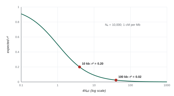
In finite populations, drift continually creates new LD while recombination removes it. John Sved showed in 1971 that the balance gives an expected squared correlation of approximately:
(with a small additional term of about 1/n from sampling). LD thus extends further in populations with small effective size. Humans of recent African ancestry, with larger long-term N_e, show shorter LD than populations that passed through the out-of-Africa bottleneck. Domestic animals and crops, which experienced strong bottlenecks and artificial selection, show LD extending over hundreds of kilobases or more, so far fewer markers are needed for association studies in cattle or maize breeding than in humans.
Recombination maps and haplotype blocks
Recombination is not uniform along chromosomes. In humans and many other mammals, most crossovers occur in narrow hotspots, one to two kilobases wide and spaced tens of kilobases apart, whose positions are specified by the DNA-binding protein PRDM9. Between hotspots, LD can extend unbroken over tens of kilobases, producing a block-like pattern in which sets of SNPs are strongly correlated. A few SNPs, called tag SNPs, can capture most of the common variation in a block. This structure, cataloged in the HapMap and 1000 Genomes projects, is what made genotyping arrays with a few hundred thousand SNPs, combined with imputation of untyped variants from reference panels, an efficient basis for genome-wide association studies.
Haplotypes are rarely observed directly, because standard genotyping does not record which alleles are on the same chromosome. A double heterozygote, Aa Bb, could carry AB and ab or Ab and aB. Haplotype frequencies are estimated with the EM algorithm, by the same logic used for ABO in lesson 2: the expected split of double heterozygotes is computed from current haplotype frequencies, and the frequencies are then updated by counting. Modern phasing programs use reference panels and the shared segments among many individuals to phase whole chromosomes with high accuracy.
Worked problem
Splitting double heterozygotes in an EM step
Current haplotype frequency estimates are p_AB = 0.5, p_Ab = 0.1, p_aB = 0.1 and p_ab = 0.3. How are 40 double heterozygotes split in the E step?
Show solution
- Phase 1 (AB/ab) has relative probability 2 × 0.5 × 0.3 = 0.30.
- Phase 2 (Ab/aB) has relative probability 2 × 0.1 × 0.1 = 0.02.
- Fraction in phase 1 = 0.30/0.32 ≈ 0.94; expected 37.5 individuals.
- Phase 2: 40 − 37.5 = 2.5 individuals.
Answer: About 37.5 are assigned AB/ab and 2.5 Ab/aB; the counts then contribute to the next haplotype frequency estimates.
Selective sweeps and genetic hitchhiking
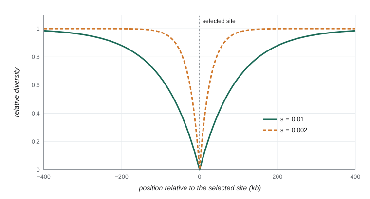
When a new beneficial mutation rises rapidly to fixation, it carries with it the stretch of chromosome on which it arose. Neutral alleles linked to the beneficial one hitchhike to high frequency, a process John Maynard Smith and John Haigh described in 1974. After a complete sweep, diversity is sharply reduced near the selected site and recovers with distance as recombination during the sweep allows linked sites to escape onto other backgrounds. The width of the region affected scales roughly with s/c: strong selection and low recombination produce wide valleys of reduced diversity. A useful approximation for the proportion of neutral diversity remaining at recombination distance c from a completed sweep is:
For N_e = 10,000 and s = 0.01, diversity is reduced by half at about c = 0.0006, roughly 60 kilobases at one centimorgan per megabase, and the valley extends over a few hundred kilobases. A sweep also leaves other signatures: an excess of rare variants as new mutations accumulate after the sweep (negative Tajima’s D), an excess of high-frequency derived alleles at the edges of the valley, and, while the sweep is still incomplete, an unusually long haplotype carrying the favored allele surrounded by little variation.
import numpy as np

Ne = 10000
for s in (0.01, 0.002):
    for kb in (10, 50, 100, 200, 400):
        c = kb * 1e-5                                   # 1 cM per Mb = 1e-5 per kb
        remaining = 1 - (2 * Ne * s) ** (-2 * c / s)
        print(f"s = {s:<6}  {kb:4d} kb from the sweep: diversity = {max(remaining, 0):.2f} of neutral")
    c_half = s * np.log(2) / (2 * np.log(2 * Ne * s))    # solve (2Ns)^(-2c/s) = 0.5
print(f" half of diversity restored at about {c_half / 1e-5:.0f} kb")s = 0.01 10 kb from the sweep: diversity = 0.10 of neutral
s = 0.01 50 kb from the sweep: diversity = 0.41 of neutral
s = 0.01 100 kb from the sweep: diversity = 0.65 of neutral
s = 0.01 200 kb from the sweep: diversity = 0.88 of neutral
s = 0.01 400 kb from the sweep: diversity = 0.99 of neutral
half of diversity restored at about 65 kb
s = 0.002 10 kb from the sweep: diversity = 0.31 of neutral
s = 0.002 50 kb from the sweep: diversity = 0.84 of neutral
s = 0.002 100 kb from the sweep: diversity = 0.97 of neutral
s = 0.002 200 kb from the sweep: diversity = 1.00 of neutral
s = 0.002 400 kb from the sweep: diversity = 1.00 of neutral
half of diversity restored at about 19 kbDetecting incomplete and soft sweeps
Before a sweep is complete, the favored allele sits on a long, nearly invariant haplotype, while chromosomes carrying the ancestral allele show normal diversity and short LD. Pardis Sabeti and colleagues formalized this with extended haplotype homozygosity (EHH) in 2002: the probability that two chromosomes carrying a given core allele are identical over a region extending a given distance from the core. Benjamin Voight and colleagues’ integrated haplotype score (iHS), from 2006, compares the area under the EHH curve for the derived and ancestral alleles, standardized across the genome by allele frequency; extreme values flag candidate sweeps.
The best-studied human example is lactase persistence, the continued production of the enzyme lactase into adulthood. In many populations of northern European ancestry, persistence is associated with a variant about 14 kilobases upstream of the lactase gene, LCT, which sits on a haplotype that extends unusually far for its frequency, a sign of rapid recent increase. Several different variants with the same effect have been found in pastoralist populations of East Africa and the Middle East, an example of convergent evolution at the molecular level and of a soft sweep at the level of the phenotype. Ancient DNA has shown that the European variant was rare until the last few thousand years, well after the start of dairying, which suggests that its rise may also have been driven by famine and disease, not simply by the availability of milk.
Not all adaptation involves new mutations sweeping from a single copy. A soft sweep occurs when selection acts on an allele that is already present on several haplotypes, either because it was segregating as standing variation or because it arose repeatedly by recurrent mutation. Soft sweeps leave weaker signatures: diversity is reduced less, because several haplotypes rise together. Polygenic adaptation, in which small shifts in allele frequency at many loci change a quantitative trait, leaves almost no sweep signature at all and must be detected with methods described in lessons 10 and 11.
Background selection and linked selection
Purifying selection against deleterious mutations also reduces linked neutral diversity, a process Brian Charlesworth and colleagues named background selection in 1993. Every time a chromosome carrying a new harmful mutation is eliminated, linked neutral variants are removed with it. The effect is strongest in regions of low recombination and high gene density. Together, sweeps and background selection, known as linked selection, explain the strong positive correlation between recombination rate and neutral diversity observed in Drosophila, humans and many other species. Because linked selection is more efficient in large populations, it also helps resolve Lewontin’s paradox from lesson 1: species with huge census sizes have less diversity than neutral theory predicts because selection at linked sites keeps reducing it.
Common mistakes
MistakeTreating |D′| = 1 as evidence that one marker is a good proxy for another.
InsteadD′ = 1 only means a haplotype is missing; proxy quality depends on r².
MistakeAssuming LD exists only between linked loci.
InsteadDrift, admixture, population structure and selection create LD even between unlinked loci, though it decays quickly.
MistakeExpecting the same marker density to work for association studies in every species.
InsteadLD extent depends on N_e and history; cattle and maize need far fewer markers than humans.
MistakeInterpreting every region of low diversity as a selective sweep.
InsteadBackground selection and low recombination also reduce diversity; compare with expectations given recombination and gene density.
MistakeExpecting soft sweeps and polygenic adaptation to leave classic sweep signatures.
InsteadSelection on several haplotypes or on many small-effect loci leaves weak or no local signatures.
Summary and key terms
- Linkage disequilibrium D = p_AB − p_A p_B measures association between alleles at different loci; D′ and r² standardize it.
- Recombination erodes LD as D_t = D_0(1 − c)^t; drift creates it, giving E[r²] ≈ 1/(1 + 4N_e c).
- Recombination hotspots produce haplotype blocks; tag SNPs and imputation exploit LD in association studies.
- A hard sweep removes linked diversity over a region that scales with s/c and leaves long haplotypes while incomplete.
- EHH and iHS detect incomplete sweeps; lactase persistence is a classic human example with convergent variants.
- Background selection and sweeps together reduce diversity most in regions of low recombination.
- linkage disequilibrium
- Non-random association of alleles at different loci.
- haplotype
- The combination of alleles carried on one chromosome.
- D′
- Lewontin’s standardized LD, D divided by its maximum given allele frequencies.
- r²
- The squared correlation between alleles at two loci.
- recombination hotspot
- A short region where crossovers are concentrated.
- tag SNP
- A SNP that captures variation at nearby correlated SNPs.
- genetic hitchhiking
- The rise in frequency of neutral alleles linked to a favored allele.
- selective sweep
- Fixation or near fixation of a favored allele and the resulting reduction of linked diversity.
- soft sweep
- A sweep in which the favored allele rises on several haplotypes at once.
- background selection
- Reduction of linked neutral diversity caused by removal of deleterious mutations.
Practice problems
Work each problem on paper first, then reveal the answer to check.
p_AB = 0.4, p_A = 0.5 and p_B = 0.6. What is D?
Show answer
0.4 − 0.3 = 0.10.
For the same values, what is the maximum possible positive D?
Show answer
min(0.5 × 0.4, 0.5 × 0.6) = 0.20, so D′ = 0.5.
Calculate r² for the same values.
Show answer
0.01/(0.5 × 0.5 × 0.6 × 0.4) = 0.01/0.06 ≈ 0.167.
With n = 300 haplotypes and r² = 0.05, what is the chi-square statistic?
Show answer
300 × 0.05 = 15.
How many generations does it take for LD between unlinked loci to fall to 1/8 of its starting value?
Show answer
Three (it halves each generation).
What is E[r²] for N_e = 5,000 and c = 0.0001?
Show answer
1/(1 + 2) ≈ 0.33.
Why do domestic species have more extended LD than humans?
Show answer
Strong bottlenecks and artificial selection reduced N_e, so drift creates more LD.
What fraction of diversity remains at c = 0.002 from a sweep with N_e = 10,000 and s = 0.01?
Show answer
1 − 200^(−0.4) ≈ 1 − 0.12 = 0.88.
What pattern does iHS look for?
Show answer
An allele on haplotypes that are unusually long relative to its frequency, compared with the other allele.
Why is neutral diversity correlated with recombination rate?
Show answer
Linked selection removes more diversity where recombination is low.
Lesson quiz · 5 questions
Score 60% or more to complete this lesson.
Create a free account to save your progress, take quizzes and earn a certificate.