
BIOL-322 · Lesson 4 of 12 · 28 min
Genetic drift and effective population size
Genetic drift is the change in allele frequency caused by the random sampling of gene copies in a finite population. BIOL-321 introduced the Wright–Fisher model, the decay of heterozygosity at rate 1/2N per generation, the standard formulas for effective population size and the result that a neutral allele is fixed with probability equal to its frequency. This lesson takes the mathematics further. We treat drift as a stochastic process with a variance that grows over time, compute exact absorption probabilities and times with a transition matrix, compare the Wright–Fisher and Moran models, distinguish different kinds of effective size, and learn how N_e is estimated from genetic data in real populations, the step that turns theory into a conservation tool.
Drift as a stochastic process
In the Wright–Fisher model, a diploid population of N individuals has 2N gene copies. Each generation, the number of copies of allele A is a binomial draw with 2N trials and success probability equal to the current frequency p. The expected frequency next generation is p, so drift has no direction, but the variance of the change is p(1 − p)/2N. Over many generations these variances accumulate. Starting from p_0, the variance of the frequency among replicate populations after t generations is:
At t = 0 the variance is zero; as t grows it approaches p_0(1 − p_0), the variance of a population that is either fixed for A (with probability p_0) or for a (with probability 1 − p_0). This formula has a second interpretation. If a species is divided into many isolated subpopulations of size N, all founded at frequency p_0, the variance among them grows exactly this way. Lesson 7 will define F_ST as this variance scaled by p_0(1 − p_0), so under pure drift F_ST = 1 − (1 − 1/2N)^t, the same quantity as the loss of heterozygosity within each subpopulation. Drift within populations and differentiation among them are two faces of one process.
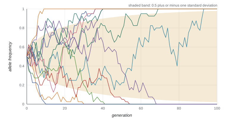
Exact results from the transition matrix
Because the number of copies next generation depends only on the number now, the Wright–Fisher model is a Markov chain with 2N + 1 states, from 0 copies to 2N. The entry in row i and column j of its transition matrix is the binomial probability of moving from i to j copies. The states 0 and 2N are absorbing: once an allele is lost or fixed, drift alone cannot bring variation back. With the matrix in hand, we can compute exact probabilities of fixation and expected times to absorption, without simulation and without approximations. For small populations, such as captive breeding groups, these exact results are directly useful.
import numpy as np
from scipy.stats import binom

N = 10; M = 2 * N                                # 20 gene copies
states = np.arange(M + 1)
P = np.array([binom.pmf(states, M, i / M) for i in states])   # transition matrix

# fixation probabilities: iterate the chain for many generations from each start
Pt = np.linalg.matrix_power(P, 2000)
fix = Pt[:, M]
print("start copies  P(fix)  equals p?")
for i in (1, 5, 10, 15):
    print(f"{i:12d}  {fix[i]:.4f}  {abs(fix[i] - i / M) < 1e-6}")

# expected time to absorption from transient states: t = (I - Q)^-1 1
Q = P[1:M, 1:M]
t = np.linalg.solve(np.eye(M - 1) - Q, np.ones(M - 1))
for i in (1, 10):
    p = i / M
    approx = -4 * N * (p * np.log(p) + (1 - p) * np.log(1 - p))   # Kimura-Ohta
print(f"start at p = {p:.2f}: exact mean time to absorption = {t[i-1]:.1f}, diffusion approx = {approx:.1f}")start copies P(fix) equals p?
1 0.0500 True
5 0.2500 True
10 0.5000 True
15 0.7500 True
start at p = 0.05: exact mean time to absorption = 7.2, diffusion approx = 7.9
start at p = 0.50: exact mean time to absorption = 26.2, diffusion approx = 27.7The exact calculation confirms that the fixation probability of a neutral allele equals its starting frequency. It also checks a classic result of Motoo Kimura and Tomoko Ohta, derived from the diffusion approximation, which treats allele frequency as varying continuously. The expected time until an allele at frequency p is either lost or fixed is about −4N[p ln p + (1 − p) ln(1 − p)] generations. Even in a population of only ten individuals the approximation is close.
Times to fixation and loss
Kimura and Ohta also derived the expected time to fixation for alleles that do become fixed. For a new neutral mutation, starting as a single copy, the conditional time to fixation is about 4N generations, while the expected time to loss, for the much larger number of mutations that are lost, is only about 2 ln(2N) generations. The contrast is striking: in a population of 10,000, a new neutral mutation that is lost survives on average about 20 generations, but one that fixes takes on the order of 40,000 generations. Most new mutations flicker briefly and vanish; the few that succeed take a very long time. This explains why most polymorphisms in a sample are young and rare, while the rare old ones that reach intermediate frequency carry information about deep history.
| Quantity | Formula (neutral) | N_e = 100 | N_e = 10,000 |
|---|---|---|---|
| Heterozygosity lost per generation | 1/(2N_e) | 0.5% | 0.005% |
| Generations to lose half of H | about 1.39 N_e | 139 | 13,900 |
| Fixation probability, new mutation | 1/(2N_e) | 0.005 | 0.00005 |
| Mean time to fixation, new mutation (if it fixes) | about 4N_e | 400 | 40,000 |
| Mean time to loss, new mutation (if lost) | about 2 ln(2N_e) | about 11 | about 20 |
Wright–Fisher and Moran models
The Wright–Fisher model assumes discrete, non-overlapping generations. In the Moran model, often used for organisms with overlapping generations and in the mathematics of the coalescent, one individual is chosen at random to reproduce and one to die at each time step. A Moran population of N haploid individuals experiences drift twice as fast per generation (N time steps) as a Wright–Fisher population of the same size, because the variance in offspring number is twice as large. In other words, a Moran population of size N behaves like a Wright–Fisher population of size N/2. This is a first glimpse of the most important idea in the lesson: what matters for drift is not the census size but the variance in reproductive success.
What effective size really measures
The effective population size, N_e, is the size of an idealized Wright–Fisher population that would show the same amount of drift as the real one. ‘The same amount of drift’ can be measured in different ways, and they do not always agree. The inbreeding effective size matches the rate of increase in inbreeding, or equivalently the loss of heterozygosity, and depends on the number of parents in the previous generation. The variance effective size matches the variance in allele frequency change from one generation to the next and depends on the number of offspring produced. In a stable population the two coincide; in a growing or shrinking population they can differ substantially. The coalescent effective size, used in lesson 6, matches the rate at which gene lineages find common ancestors and is the quantity estimated from DNA sequence diversity.
A general expression for a population of N parents, where V_k is the variance in the number of gene copies each contributes to the next generation, shows the central role of reproductive variance:
When family sizes follow a Poisson distribution with mean 2 (V_k = 2), N_e ≈ N, which is the ideal case. When some individuals have many offspring and most have none, as in species with high fecundity and high early mortality, V_k can be enormous and N_e tiny relative to N. Marine fishes and oysters, with millions of eggs per female and survival governed by chance currents, sometimes show N_e/N ratios below 10⁻³, a phenomenon called sweepstakes reproduction. In the other direction, captive breeding programs that equalize family sizes, so that every pair contributes exactly two offspring (V_k = 0), achieve N_e ≈ 2N, twice the census size. This is why zoo and hatchery managers try to equalize contributions among founders.
Worked problem
Equalizing family size in a captive program
A captive population of 30 breeding adults is managed so that each adult contributes exactly two offspring to the next breeding generation. In the wild population of 30, the variance in offspring number per individual is 6. Compare the effective sizes.
Show solution
- Captive: V_k = 0, so N_e = (4 × 30 − 2)/(0 + 2) = 118/2 = 59.
- Wild: V_k = 6, so N_e = 118/(6 + 2) = 14.75.
- Heterozygosity lost per generation: 1/(2 × 59) ≈ 0.85 percent captive, 1/(2 × 14.75) ≈ 3.4 percent wild.
- Over 10 generations, the captive group retains (1 − 1/118)^10 ≈ 92 percent of its heterozygosity, the wild group (1 − 1/29.5)^10 ≈ 71 percent.
Answer: N_e ≈ 59 in the managed group and about 15 in the wild group of the same census size; equalizing contributions quadruples N_e here.
Estimating effective size from genetic data
Census counts are not enough, so conservation geneticists estimate N_e directly from genetic data. Three families of methods are widely used.
The temporal method compares allele frequencies in samples taken several generations apart. Because drift causes frequencies to change with variance proportional to t/2N_e, the standardized variance in frequency change, F, estimates t/(2N_e) after correcting for the noise added by sampling S_0 and S_t individuals at each time. The estimate is then N_e = t / [2(F − 1/(2S_0) − 1/(2S_t))]. Museum specimens and archived scales or tissue make this method possible for many species.
The linkage disequilibrium method uses a single sample. In a finite population, drift creates random associations between alleles at different loci, and for unlinked loci the expected squared correlation is about 1/(3N_e) plus a sampling term of about 1/S. Subtracting the sampling term and inverting gives an estimate of N_e for the parental generation. This approach, implemented in the program NeEstimator, is now the most widely used single-sample method. Lesson 9 explains linkage disequilibrium in detail.
Sibship and pedigree methods reconstruct family relationships from multilocus genotypes; the more often random pairs of individuals turn out to be siblings, the smaller the number of breeders that produced them. Finally, coalescent methods use sequence diversity to estimate long-term N_e and, through changes in the site frequency spectrum or in the density of coalescent events across the genome, to reconstruct how N_e has changed over thousands of generations.
import numpy as np
rng = np.random.default_rng(322)

Ne_true, t, L = 150, 6, 400                 # effective size, generations apart, loci
S0 = St = 60                                # individuals sampled at each time
p0 = rng.uniform(0.1, 0.9, L)
p = p0.copy()
for _ in range(t):
    p = rng.binomial(2 * Ne_true, p) / (2 * Ne_true)

x = rng.binomial(2 * S0, p0) / (2 * S0)     # sample frequencies at time 0
y = rng.binomial(2 * St, p) / (2 * St)      # sample frequencies at time t
z = (x + y) / 2
keep = (z > 0.05) & (z < 0.95)
Fc = np.mean((x[keep] - y[keep])**2 / (z[keep] * (1 - z[keep])))
Ne_hat = t / (2 * (Fc - 1 / (2 * S0) - 1 / (2 * St)))
print(f"standardized variance F = {Fc:.4f}")
print(f"temporal estimate of Ne = {Ne_hat:.0f} (true value {Ne_true})")standardized variance F = 0.0345 temporal estimate of Ne = 168 (true value 150)
The estimate lands near the true value, but the confidence intervals on N_e estimates are typically wide, especially when N_e is large relative to the number of generations and individuals sampled, because the drift signal is then small compared with sampling noise. A general rule of genetic estimation of N_e is that small effective sizes, the ones of greatest conservation concern, are estimated most precisely.
Ratios of effective to census size and conservation rules of thumb
Reviews of hundreds of estimates, beginning with Richard Frankham’s in 1995, found that N_e for wildlife populations is typically around one tenth of census size, with very wide variation among species. Fluctuations in population size, unequal sex ratios and variance in family size each contribute, and they compound one another. A population of 1,000 animals may therefore lose variation like a population of 100.
These numbers feed into the ‘50/500’ rule proposed in 1980: an effective size of at least 50 to avoid inbreeding depression in the short term, and 500 to retain enough additive genetic variance for long-term adaptation. Frankham and colleagues argued in 2014 that these figures are too low and proposed at least 100 and 1,000, respectively, a revision since adopted in some assessments of genetic diversity in conservation policy. Because N_e is typically a fraction of N, an effective size of 1,000 can require several thousand adults. The Kunming–Montreal Global Biodiversity Framework of 2022 includes a headline indicator based on the proportion of populations within species that have N_e above 500, which has made effective-size estimation part of national biodiversity reporting.
Common mistakes
MistakeEquating effective size with the number of animals counted.
InsteadN_e reflects variance in reproductive success, sex ratio and fluctuations in size; it is usually much smaller than N.
MistakeAssuming that drift has no effect in a population of several thousand.
InsteadDrift acts on N_e, not N; species with sweepstakes reproduction can have tiny N_e despite huge numbers.
MistakeThinking that a new mutation that fixes by drift does so quickly.
InsteadConditional on fixation, a new neutral mutation takes about 4N_e generations; lost mutations disappear within a few dozen.
MistakeForgetting to subtract sampling noise in the temporal method.
InsteadSampling individuals adds variance of about 1/(2S) per sample; without correction, N_e is underestimated.
MistakeTreating inbreeding and variance effective sizes as always equal.
InsteadThey coincide only in stable populations; in growing or declining populations they can differ greatly.
Summary and key terms
- Drift is a binomial sampling process whose variance accumulates as Var(p_t) = p_0(1 − p_0)[1 − (1 − 1/2N)^t].
- The Wright–Fisher model is a Markov chain; its transition matrix gives exact fixation probabilities and absorption times.
- A new neutral mutation that fixes takes about 4N_e generations; most new mutations are lost within about 2 ln(2N_e) generations.
- Effective size depends on the variance in reproductive success: N_e = (4N − 2)/(V_k + 2).
- N_e can be estimated by temporal, linkage disequilibrium, sibship and coalescent methods; small N_e is estimated most precisely.
- N_e is typically around a tenth of census size; conservation guidelines now aim for N_e of at least 100 in the short term and 1,000 in the long term.
- genetic drift
- Random change in allele frequency caused by sampling of gene copies in a finite population.
- Markov chain
- A random process in which the next state depends only on the current state.
- absorbing state
- A state that cannot be left once entered, such as loss or fixation of an allele.
- diffusion approximation
- Treating allele frequency as a continuous variable to derive approximate results for drift and selection.
- Moran model
- A model of overlapping generations in which one individual reproduces and one dies at each step.
- inbreeding effective size
- The ideal population size with the same rate of increase in inbreeding.
- variance effective size
- The ideal population size with the same variance in allele frequency change.
- sweepstakes reproduction
- Very high variance in reproductive success, as in many marine species, which greatly reduces N_e.
- temporal method
- Estimating N_e from the change in allele frequencies between samples taken generations apart.
- 50/500 rule
- A guideline for minimum effective sizes to avoid inbreeding depression and retain adaptive potential, since revised upward.
Practice problems
Work each problem on paper first, then reveal the answer to check.
A population of N = 25 starts at p_0 = 0.4. What is the variance in p after 50 generations?
Show answer
0.24 × [1 − (0.98)^50] ≈ 0.24 × 0.636 ≈ 0.153.
What is the long-run limit of that variance, and what does it mean?
Show answer
0.24, the variance when each population is fixed for A with probability 0.4 and lost otherwise.
How many generations does a new neutral mutation take to fix, on average, if N_e = 2,500?
Show answer
About 4N_e = 10,000 generations.
About how long does a new neutral mutation that is lost survive if N_e = 2,500?
Show answer
About 2 ln(5,000) ≈ 17 generations.
A Moran population has N = 200 haploid individuals. What Wright–Fisher size gives the same drift?
Show answer
About 100.
In a stable population of 50 with Poisson family sizes, what is N_e?
Show answer
V_k = 2, so N_e = (200 − 2)/4 ≈ 50.
What is N_e for 50 parents if family sizes are equalized?
Show answer
(200 − 2)/2 = 99.
In the temporal method, F = 0.03 after 5 generations with 50 individuals sampled each time. Estimate N_e.
Show answer
F − 0.01 − 0.01 = 0.01; N_e = 5/(2 × 0.01) = 250.
Why are large N_e values estimated imprecisely?
Show answer
The drift signal becomes small relative to sampling noise.
What effective size targets did Frankham and colleagues propose in 2014?
Show answer
At least 100 to avoid inbreeding depression and 1,000 to retain adaptive potential.
Lesson quiz · 5 questions
Score 60% or more to complete this lesson.
Create a free account to save your progress, take quizzes and earn a certificate.