
BIOL-322 · Lesson 1 of 12 · 30 min
Genetic variation and its measurement
Population genetics is the study of genetic variation within and between populations and of the forces that change it: mutation, selection, drift, gene flow and recombination. Earlier courses introduced these forces one at a time. BIOL-108 showed that alleles can be counted and that drift is stronger in small populations; BIOL-201 used Hardy–Weinberg proportions as a check on genotype data; BIOL-321 placed selection, drift and gene flow inside the wider story of evolution. This course treats population genetics as a quantitative science in its own right. It builds the mathematical models, shows how they are fitted to real data, and explains how the same few ideas are used in conservation, forensic science, plant and animal breeding and human genetics.
Every model in the course rests on measurement. Before asking why a population has the variation it has, we need to describe that variation precisely: what kinds of differences exist in the genome, how they are scored, which summary numbers capture them, and how much those numbers would change if we had sampled different individuals. This first lesson sets out that toolkit.
What varies in a genome
Genetic variation is any difference in DNA sequence among the gene copies carried by members of a population. The simplest and most abundant kind is the single-nucleotide polymorphism, or SNP, a site at which some copies carry one base and others carry another. Most SNPs have just two alleles because the per-site mutation rate is so low that a second mutation at the same site is rare. Short insertions and deletions (indels) add or remove a few bases. Short tandem repeats, also called microsatellites, are runs of a short motif such as GATA repeated a variable number of times; they mutate thousands of times faster than single bases and so often have many alleles. Larger structural variants include copy-number variants, in which a stretch of DNA from about a thousand bases to several million is duplicated or deleted, inversions, and translocations.
| Kind of variant | Typical size | Typical number of alleles | Mutation rate (per locus per generation) | Common uses |
|---|---|---|---|---|
| SNP | 1 base | 2 | about 10⁻⁸ | Genome scans, GWAS, ancestry, demographic inference |
| Short indel | 1–50 bases | 2 | about 10⁻⁹ | Variant calling, disease genetics |
| Microsatellite (STR) | 2–6 base motif, repeated | 5–30 or more | 10⁻⁴ to 10⁻³ | Forensic profiles, parentage, wildlife genetics |
| Copy-number variant | 1 kb to several Mb | 2 or more | Variable, often high | Gene dosage, disease, adaptation |
| Inversion | 1 kb to many Mb | 2 | Low | Suppression of recombination, local adaptation |
These classes matter because they behave differently under the models we will build. A marker with a high mutation rate, such as an STR, reaches equilibrium between mutation and drift quickly and carries many alleles, which makes it powerful for telling individuals apart but less useful for dating events far in the past. SNPs are nearly always biallelic and, because there are millions of them, they dominate modern studies. The infinite-sites assumption, that every new mutation occurs at a site that has never mutated before, is a good approximation for SNPs and underlies the diversity statistics in lesson 6.
From proteins to genomes: a short history of measurement
Until the mid-1960s, population geneticists could study only variation visible as a phenotype, such as blood groups or banding patterns on snail shells. In 1966, Richard Lewontin and John Hubby used gel electrophoresis to separate protein variants (allozymes) in Drosophila pseudoobscura, and Harry Harris did the same for human enzymes. Both found far more variation than many had expected: roughly a third of loci were polymorphic, and an average individual was heterozygous at roughly a tenth of them. This finding launched a long debate over whether most variation is maintained by balancing selection or is neutral, the debate that led to Kimura’s neutral theory, which BIOL-321 introduced and lesson 5 develops further.
Electrophoresis detects only amino acid changes that alter a protein’s charge, so it underestimates variation. Restriction fragment length polymorphisms, microsatellites and direct sequencing followed. Today, whole genomes can be sequenced cheaply enough that population samples of thousands of individuals are routine, and reduced-representation methods such as RAD-seq let wildlife biologists genotype tens of thousands of SNPs in species with no reference genome. The questions have not changed much since 1966, but the data now allow them to be answered locus by locus across the whole genome.
Counting alleles and genotypes
The raw data of population genetics are genotypes. For a diploid organism and a locus with alleles A and a, each sampled individual is AA, Aa or aa. If a sample of n individuals contains n_AA, n_Aa and n_aa of each genotype, the sample allele frequency of A is the number of A copies divided by the total number of copies:
The frequency of a is q̂ = 1 − p̂. The hat reminds us that this is an estimate of the unknown population frequency, p. Because the 2n gene copies are, under random sampling, like draws from a binomial distribution, the standard error of p̂ is approximately the square root of p̂(1 − p̂)/2n. With 50 individuals (100 copies) and p̂ = 0.3, the standard error is about 0.046, so a 95 percent confidence interval runs roughly from 0.21 to 0.39. Allele frequencies estimated from small samples are imprecise, and a difference of 0.05 between two samples of 50 is well within sampling noise.
When the sample is drawn from relatives, from a structured population or from individuals chosen for a trait, the gene copies are not independent and the binomial standard error is too small. Lesson 7 shows how population structure inflates variance, and lesson 11 shows why ascertainment, the way a sample was chosen, can bias association studies.
Summary statistics of variation
Several numbers summarize the variation at a set of loci. The proportion of polymorphic loci, P, counts loci at which the most common allele has a frequency below some cut-off, often 0.95 or 0.99. It depends heavily on sample size and on the cut-off, so it is now used mostly descriptively. Allelic richness is the number of distinct alleles; it is especially sensitive to sample size because rare alleles appear only in large samples, so it is usually standardized by rarefaction to a common sample size.
The most widely used summary is expected heterozygosity, also called gene diversity: the probability that two gene copies drawn at random from the population carry different alleles. For a locus with allele frequencies p_1, p_2, … , p_k:
If the population mates at random, H_e is also the expected proportion of heterozygous individuals, which is where the name comes from. Masatoshi Nei showed that the plug-in estimate, computed from sample frequencies, is biased downward because the same copy cannot be drawn twice in a finite sample. The unbiased estimator multiplies by 2n/(2n − 1), where 2n is the number of gene copies sampled. Observed heterozygosity, H_o, is simply the proportion of sampled individuals that are heterozygous. Comparing H_o with H_e is the starting point for detecting inbreeding, population structure and genotyping errors, the subject of lessons 2 and 7.
Worked problem
Gene diversity at a microsatellite
A sample of 40 lake trout (80 gene copies) is genotyped at a microsatellite. The allele counts are 32, 24, 16 and 8 for four alleles, and 26 of the 40 fish are heterozygous. Calculate H_o, the plug-in H_e and Nei’s unbiased H_e.
Show solution
- Allele frequencies: 32/80 = 0.40, 24/80 = 0.30, 16/80 = 0.20, 8/80 = 0.10.
- Sum of squares: 0.16 + 0.09 + 0.04 + 0.01 = 0.30, so the plug-in H_e = 1 − 0.30 = 0.70.
- Unbiased H_e = (80/79) × 0.70 ≈ 0.709.
- Observed heterozygosity H_o = 26/40 = 0.65.
- H_o is a little below H_e; whether the gap is meaningful requires a test, because a sample of 40 has a lot of sampling variance.
Answer: H_o = 0.65, plug-in H_e = 0.70 and unbiased H_e ≈ 0.71. The small deficit of heterozygotes could be chance, mild inbreeding or a few null alleles, and lesson 2 shows how to test it.
Expected heterozygosity is bounded by 1 − 1/k for k alleles and is reached when all alleles are equally common. For a biallelic SNP, H_e = 2pq, which is at most 0.5. This means that heterozygosity values from microsatellites and SNPs cannot be compared directly: a microsatellite with H_e = 0.8 is not ‘more diverse’ than a SNP panel with H_e = 0.3 in any meaningful biological sense, because the two kinds of marker have very different mutation rates and allele numbers.
Nucleotide diversity
For sequence data, the natural measure is nucleotide diversity, π: the average number of differences per site between two sequences drawn at random from the sample. If n sequences of length L have been aligned, π is the sum of pairwise differences over all n(n − 1)/2 pairs, divided by the number of pairs and by L. Humans have π of roughly 0.001, meaning that two copies of a human chromosome differ at about one site in every thousand. Common chimpanzees have higher diversity than humans despite a much smaller census population, a hint that diversity reflects long-term effective size, not current numbers. Lesson 6 connects π to the coalescent and to the population mutation rate θ = 4N_eμ, and compares it with a second estimator based on the number of segregating sites.
| Species | Approximate π (per site) | Comment |
|---|---|---|
| Humans | 0.0008–0.001 | Higher in African populations than elsewhere |
| Common chimpanzee | 0.001–0.002 | Long-term effective size larger than that of humans |
| Drosophila melanogaster | 0.005–0.01 | Very large effective population size |
| Cheetah | Very low, below most mammals | Signature of ancient bottlenecks |
| Many marine invertebrates | Above 0.01 | Enormous populations and high fecundity |
A long-standing puzzle, sometimes called Lewontin’s paradox, is that diversity varies far less among species than census population size does. Insects with trillions of individuals are only about ten times more diverse than mammals with millions. Part of the answer is that diversity reflects the harmonic mean of population size over long periods, which is dominated by bottlenecks; part is that selection at linked sites, the subject of lesson 9, removes neutral diversity more efficiently in large populations.
Computing diversity with uncertainty
Summary statistics should always come with a measure of uncertainty. Because loci differ in their history, the variance of a genome-wide average comes more from differences among loci than from sampling of individuals. A convenient approach is the bootstrap: resample loci with replacement many times, recompute the statistic, and use the spread of the resampled values as a confidence interval. The code below simulates a genotype matrix for 60 diploid individuals at 500 biallelic SNPs and computes H_o, Nei’s unbiased H_e and a bootstrap interval.
import numpy as np
rng = np.random.default_rng(322)

n_ind, n_loci = 60, 500
p_true = rng.beta(0.6, 0.6, n_loci)            # allele frequencies vary among loci
G = rng.binomial(2, p_true, size=(n_ind, n_loci))  # 0, 1 or 2 copies of allele A

p_hat = G.sum(axis=0) / (2 * n_ind)
keep = (p_hat > 0) & (p_hat < 1)                # drop loci that are monomorphic in the sample
p_hat, G = p_hat[keep], G[:, keep]
two_n = 2 * n_ind

Ho = np.mean(G == 1, axis=0)
He = (two_n / (two_n - 1)) * 2 * p_hat * (1 - p_hat)
print(f"polymorphic loci: {keep.sum()} of {n_loci}")
print(f"mean Ho = {Ho.mean():.3f}, mean unbiased He = {He.mean():.3f}")

boot = []
for _ in range(2000):
    idx = rng.integers(0, len(He), len(He))
    boot.append(He[idx].mean())
lo, hi = np.percentile(boot, [2.5, 97.5])
print(f"95% bootstrap interval for mean He: {lo:.3f} to {hi:.3f}")polymorphic loci: 472 of 500 mean Ho = 0.284, mean unbiased He = 0.285 95% bootstrap interval for mean He: 0.270 to 0.300
Because the simulated individuals were drawn at random from a population in Hardy–Weinberg proportions, H_o and H_e agree closely. In real data, a consistent shortfall of heterozygotes across many loci points to inbreeding or population structure, while a shortfall at only a few loci more often reflects technical problems such as null alleles at microsatellites or poorly called SNPs.
The site frequency spectrum
Heterozygosity and π compress all the information about variation into one number. A richer summary is the site frequency spectrum (SFS): the count of polymorphic sites at which the derived (mutant) allele appears in exactly 1, 2, … , n − 1 of n sampled sequences. If we know which allele is ancestral, usually by comparison with an outgroup species, we have the unfolded spectrum. If not, we can only count the minor allele, giving the folded spectrum, which runs from 1 to n/2.
The SFS is one of the most informative summaries in population genetics. Under the standard neutral model with constant population size, the expected number of sites at which the derived allele appears i times is proportional to 1/i: singletons are the most common class, doubletons half as common, and so on. Population growth produces an excess of rare variants, because many recent mutations have arisen on the long terminal branches of a growing population’s genealogy. A bottleneck or population structure produces an excess of intermediate-frequency variants. Positive selection leaves its own distortions, including an excess of high-frequency derived alleles near a sweep. Lesson 6 derives the 1/i expectation from the coalescent; here we simply learn to compute and read the spectrum.
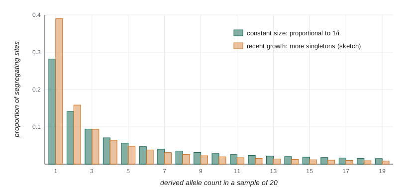
import numpy as np
rng = np.random.default_rng(3221)

n = 20
i = np.arange(1, n)
expected = (1 / i) / np.sum(1 / i)               # neutral, constant size

# simulate 2,000 segregating sites by sampling derived counts from the neutral SFS
counts = rng.choice(i, size=2000, p=expected)
observed = np.bincount(counts, minlength=n)[1:] / 2000

for k in (1, 2, 3, 5, 10, 19):
    print(f"derived count {k:2d}: expected {expected[k-1]:.3f}, observed {observed[k-1]:.3f}")

# fold the spectrum (minor allele counts 1..n/2)
folded = np.array([observed[k-1] + (observed[n-k-1] if k != n - k else 0) for k in range(1, n//2 + 1)])
print("folded spectrum, first five classes:", np.round(folded[:5], 3))derived count 1: expected 0.282, observed 0.283 derived count 2: expected 0.141, observed 0.130 derived count 3: expected 0.094, observed 0.099 derived count 5: expected 0.056, observed 0.051 derived count 10: expected 0.028, observed 0.027 derived count 19: expected 0.015, observed 0.014 folded spectrum, first five classes: [0.298 0.146 0.12 0.095 0.071]
Folding the spectrum combines derived counts i and n − i, which loses information about high-frequency derived alleles but avoids errors in assigning the ancestral state. Misassigning ancestral alleles is a real hazard: if the outgroup carries a different mutation at the same site, a rare derived allele will be miscounted as a common one, producing a false signal of selection.
From data files to frequencies
Modern genotype data usually arrive as a variant call format (VCF) file, in which each row is a variant and each column a sample, with genotypes written as 0/0, 0/1 or 1/1 and a quality score for each call. Three practical decisions shape every downstream analysis. First, low-quality genotypes and individuals with many missing calls are filtered out. Second, very rare variants are often removed with a minor allele frequency filter, because they are hard to call reliably; but because rare variants carry information about recent history, such filters distort the site frequency spectrum and must be reported. Third, loci in strong linkage disequilibrium are often thinned, because many methods assume independent loci. None of these choices is neutral, and differences in filtering explain many disagreements between published studies.
Low-coverage sequencing adds another layer of uncertainty: when a heterozygous site is covered by only two or three reads, both reads may by chance come from the same chromosome and the individual will be miscalled as a homozygote. Methods that work with genotype likelihoods instead of hard calls avoid this bias, and they are now standard for ancient DNA and for large wildlife surveys.
Common mistakes
MistakeComparing heterozygosity from microsatellites directly with heterozygosity from SNPs.
InsteadCompare like with like. Marker types differ in mutation rate and number of alleles, so their H_e values are on different scales.
MistakeReporting an allele frequency from 15 individuals as if it were exact.
InsteadGive a standard error or confidence interval; with 30 gene copies the standard error of a frequency near 0.5 is about 0.09.
MistakeUsing the plug-in H_e from a small sample.
InsteadApply Nei’s correction 2n/(2n − 1), which matters most when samples are small.
MistakeTreating a minor allele frequency filter as harmless.
InsteadReport filters, because removing rare variants distorts the site frequency spectrum and many diversity statistics.
MistakeAssuming high diversity means a large current population.
InsteadDiversity reflects long-term effective size, which bottlenecks dominate; a large population can have low diversity and vice versa.
Summary and key terms
- Genetic variation includes SNPs, indels, microsatellites and structural variants, which differ in mutation rate, allele number and use.
- Sample allele frequencies are estimates with binomial sampling error, roughly the square root of p(1 − p)/2n.
- Expected heterozygosity H_e = 1 − Σp_i² is the probability that two random gene copies differ; Nei’s correction removes small-sample bias.
- Nucleotide diversity π is the average number of pairwise differences per site; humans have π of about 0.001.
- The site frequency spectrum records how many sites have the derived allele at each count; under neutrality and constant size it is proportional to 1/i.
- Filtering, missing data and low coverage all affect summary statistics and must be reported.
- SNP
- A single-nucleotide polymorphism: a site where gene copies carry different bases.
- microsatellite
- A short tandem repeat whose number of repeat units varies among alleles.
- copy-number variant
- A duplication or deletion of a stretch of DNA that varies among individuals.
- expected heterozygosity
- The probability that two randomly chosen gene copies carry different alleles; also called gene diversity.
- observed heterozygosity
- The proportion of sampled individuals that are heterozygous.
- nucleotide diversity
- The average number of differences per site between two randomly chosen sequences.
- allelic richness
- The number of distinct alleles, usually standardized to a common sample size.
- site frequency spectrum
- The distribution of derived or minor allele counts across segregating sites.
- infinite-sites model
- The assumption that each mutation occurs at a site that has not mutated before.
- bootstrap
- Resampling the data with replacement to estimate the uncertainty of a statistic.
Practice problems
Work each problem on paper first, then reveal the answer to check.
A sample has 18 AA, 24 Aa and 8 aa individuals. What is p̂?
Show answer
(36 + 24)/100 = 0.60.
What is the approximate standard error of p̂ = 0.6 from 50 individuals?
Show answer
The square root of 0.6 × 0.4/100 is about 0.049.
Calculate H_e for a locus with frequencies 0.5, 0.25 and 0.25.
Show answer
1 − (0.25 + 0.0625 + 0.0625) = 0.625.
What is the maximum possible H_e at a biallelic SNP?
Show answer
0.5, when both alleles have frequency 0.5.
Apply Nei’s correction to a plug-in H_e of 0.40 from 10 individuals.
Show answer
(20/19) × 0.40 ≈ 0.421.
Four sequences of 100 bases differ pairwise by 2, 3, 1, 2, 4 and 0 sites. What is π?
Show answer
Mean pairwise difference = 12/6 = 2, so π = 2/100 = 0.02.
Under the standard neutral model, how do the expected numbers of singletons and doubletons compare?
Show answer
Doubletons are expected to be half as common as singletons.
What pattern in the site frequency spectrum suggests recent population growth?
Show answer
An excess of rare variants, especially singletons.
Why does folding the spectrum lose information?
Show answer
It merges derived counts i and n − i, so high-frequency derived alleles cannot be distinguished from rare ones.
Why might a heterozygote be miscalled as a homozygote in low-coverage data?
Show answer
All the few reads covering the site may come from the same chromosome by chance.
Lesson quiz · 5 questions
Score 60% or more to complete this lesson.
Create a free account to save your progress, take quizzes and earn a certificate.