
BIOL-321 · Lesson 9 of 12 · 28 min
Phylogenetics II: dating, ancestral states and the comparative method
Once we have a tree, we can use it to ask historical questions. When did lineages split? What did ancestors look like? Did a trait evolve once or many times? Are two traits correlated across species because of adaptation, or only because related species resemble each other? This lesson covers molecular dating with fossil calibrations, reconstruction of ancestral states and phylogenetic comparative methods, especially Joseph Felsenstein’s phylogenetic independent contrasts. BIOL-108 introduced the molecular clock with a single rate; here we see how calibrations, rate variation and uncertainty are handled in practice.
From branch lengths to time
Branch lengths from a likelihood analysis are in expected substitutions per site, the product of rate and time. To convert them to time, we need at least one calibration: a node whose age is known independently, usually from fossils or from geological events such as the formation of an island or the closure of the Isthmus of Panama. If substitutions accumulate at a constant rate r per lineage, the divergence d between two sequences (counting both lineages) after time T is
A fossil gives a minimum age for the node it belongs to: the oldest fossil that can be confidently placed in a clade shows that the clade existed at least by then, but the lineage may be older, because early members are rarely preserved. A maximum age is harder to justify; it may come from the absence of the group in well-sampled older rocks. Modern dating methods therefore treat calibrations as probability distributions, for example a lognormal distribution with a hard minimum at the fossil age and a soft upper tail.
Worked problem
Calibrating a clock with a fossil
Two bird species differ at 6.4 % of sites in a mitochondrial gene (corrected distance). A pair of related species in the same genus, whose split is calibrated by a fossil at 4.0 million years, differs by 8.0 %. Assuming a clock, estimate the rate and the age of the first split.
Show solution
- Rate per lineage: r = d/(2T) = 0.080/(2 × 4.0) = 0.010 substitutions per site per million years, or 1 % per lineage per million years.
- Age of the first split: T = 0.064/(2 × 0.010) = 3.2 million years.
- Because the fossil gives only a minimum age for the calibration node, the true rate could be lower and all ages older; the estimate of 3.2 million years is best treated as a minimum under these assumptions.
Answer: About 3.2 million years, with the caveat that fossil calibrations are minimum ages.
The often-quoted rate of about 2 % divergence per million years for bird mitochondrial cytochrome b, which is 1 % per lineage, illustrates a calibrated rate, but rates differ among genes, lineages and timescales, and rates estimated over short timescales are often higher, because slightly harmful mutations that will eventually be removed are still present.
Relaxed clocks and uncertainty
Rates of molecular evolution vary across the tree of life. Small-bodied animals with short generation times, such as rodents, tend to have faster rates per year than large-bodied ones such as whales and elephants; rates also depend on metabolic rate, DNA repair and population size. Relaxed clock models allow rates to vary among branches, either independently from a distribution (uncorrelated relaxed clock) or with rates on neighboring branches correlated (autocorrelated clock). Bayesian programs such as BEAST and MCMCTree estimate tree, rates and node ages jointly, combining sequence data with calibration priors, and report 95 % highest posterior density (HPD) intervals.
Calibration uncertainty usually dominates the error in deep divergence dates: adding more sequence data does not reduce uncertainty that arises from not knowing the exact age of the calibration node. The following simulation propagates both sources of uncertainty for a simple two-node problem.
import numpy as np
rng = np.random.default_rng(321)
n = 100_000
# Calibration node: fossil minimum 50 Myr, true age drawn as 50 + lognormal offset (median about 5 Myr)
cal_age = 50 + rng.lognormal(mean=np.log(5), sigma=0.6, size=n)
d_cal = rng.normal(0.300, 0.010, n)       # divergence at calibration node (substitutions per site, both lineages)
d_target = rng.normal(0.120, 0.008, n)    # divergence at the node we want to date
rate = d_cal / (2 * cal_age)              # per-lineage rate
age = d_target / (2 * rate)
lo, med, hi = np.percentile(age, [2.5, 50, 97.5])
print(f"target node age: median {med:.1f} Myr, 95% interval {lo:.1f} to {hi:.1f} Myr")
# How much of the spread is due to calibration uncertainty?
age_fixed_cal = d_target / (2 * (d_cal / (2 * np.median(cal_age))))
lo2, hi2 = np.percentile(age_fixed_cal, [2.5, 97.5])
print(f"with calibration age fixed at its median: 95% interval {lo2:.1f} to {hi2:.1f} Myr")target node age: median 22.2 Myr, 95% interval 18.6 to 27.6 Myr with calibration age fixed at its median: 95% interval 18.9 to 25.3 Myr
Fixing the calibration age narrows the interval by about a third and removes most of its long upper tail, showing that much of the uncertainty, especially toward older dates, comes from the fossil record rather than the sequences. In real studies with thousands of sites, sequence error shrinks further while calibration error does not. An alternative approach, tip dating or the fossilized birth–death model, includes fossils as tips with morphological data, rather than only as calibrations on nodes, using information from all relevant fossils rather than only the oldest.
Molecular dates have sometimes conflicted with the fossil record. Early molecular studies suggested that many modern bird and mammal orders originated deep in the Cretaceous, long before their first fossils, whereas the fossil record shows an explosive radiation of placental mammals and neornithine birds after the end-Cretaceous extinction 66 million years ago. With better models and calibrations, the gap has narrowed: many analyses now place the origin of placental orders close to the boundary, though the deepest splits among placental mammals are still often estimated to predate it.
Reconstructing ancestral states
Given a tree and the states of a character at the tips, we can infer the likely states at internal nodes. Parsimony reconstruction assigns states that minimize the number of changes, using the Fitch algorithm (Lesson 8) followed by a pass from root to tips. Likelihood reconstruction uses a model of change, for a discrete character typically the Mk model, in which a character with k states changes between states at rate q, and gives the probability of each state at each node. For continuous characters, the standard model is Brownian motion: the trait changes by random increments with variance proportional to time, so the expected change is zero and the variance after time t is σ²t.
import numpy as np
from scipy.linalg import expm
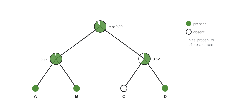
# Marginal ancestral state at the root of a four-taxon tree for a binary trait (0 = absent, 1 = present)
# Tree ((A:1,B:1):1,(C:1,D:1):1); tips A=1, B=1, C=0, D=1 (invented)
def P(t, q):
    Qm = np.array([[-q, q], [q, -q]])
    return expm(Qm * t)
def cond(tip):
    v = np.zeros(2); v[tip] = 1; return v
def node(lv, rv, tl, tr, q):
    return (P(tl, q) @ lv) * (P(tr, q) @ rv)
for q in (0.1, 0.5, 2.0):
    ab = node(cond(1), cond(1), 1, 1, q)
    cd = node(cond(0), cond(1), 1, 1, q)
    root = node(ab, cd, 1, 1, q)
    post = root * 0.5 / (root * 0.5).sum()          # equal prior on root states
print(f"rate q = {q}: P(root = present) = {post[1]:.3f}, log-likelihood = {np.log((root*0.5).sum()):.3f}")rate q = 0.1: P(root = present) = 0.901, log-likelihood = -3.369 rate q = 0.5: P(root = present) = 0.619, log-likelihood = -2.791 rate q = 2.0: P(root = present) = 0.500, log-likelihood = -2.773
When change is slow, the root is almost certainly in the state shared by most tips. When change is fast, the tips carry little information about the deep past and the reconstruction approaches 50 %. In practice, q is estimated from the data by maximum likelihood. Reconstructions are only as good as the model; if a trait is easier to lose than to gain, as with complex structures such as eyes in cave animals or wings in insects, a symmetrical model may mislead. Asymmetric models allow different gain and loss rates. Ancestral reconstruction has been used to infer that the ancestor of placental mammals was a small insectivore, to study repeated evolution of viviparity in squamate reptiles and even to resurrect ancestral proteins in the laboratory, such as ancestral steroid receptors studied by Joseph Thornton’s group.
The comparative method
The comparative method tests hypotheses about adaptation by looking for correlations between traits, or between traits and environments, across species. For example, do primates with larger groups have larger brains? Do birds in colder climates have larger bodies, as Bergmann’s rule predicts? A key problem is that species are not independent data points. Closely related species share traits because they inherited them from a common ancestor, not because each evolved them independently. Treating species as independent inflates the apparent sample size and can produce spurious correlations.
Felsenstein illustrated the problem in 1985. Imagine two clades of species, each of which inherited a combination of large body size and long life from its own ancestor. Across all species, size and lifespan appear tightly correlated, but in fact there may have been only one evolutionary event in each clade. His solution, phylogenetic independent contrasts (PIC), calculates differences between sister taxa (or nodes) at each split in the tree. Because each contrast reflects evolution along separate branches since a split, contrasts are statistically independent under Brownian motion. Each contrast is standardized by dividing by the square root of the sum of its branch lengths, the expected standard deviation of change, and the correlation between traits is then calculated across contrasts, with a regression forced through the origin.
import numpy as np
rng = np.random.default_rng(321)
# Two clades of 16 species each; the deep split is long, splits within clades are short.
# Two traits evolve INDEPENDENTLY by Brownian motion. Does an ordinary regression find a relationship?
def simulate():
    x = np.empty(32); y = np.empty(32)
    for clade in range(2):
        bx, by = rng.normal(0, 3), rng.normal(0, 3)           # change along the long deep branch
        x[clade*16:(clade+1)*16] = bx + rng.normal(0, 0.5, 16)  # short within-clade change
        y[clade*16:(clade+1)*16] = by + rng.normal(0, 0.5, 16)
    return x, y
def pval(r, n):
    from scipy import stats
    t = r*np.sqrt((n - 2)/(1 - r**2)); return 2*stats.t.sf(abs(t), n - 2)
reps, naive_sig, contrast_sig = 2000, 0, 0
for _ in range(reps):
    x, y = simulate()
    r_naive = np.corrcoef(x, y)[0, 1]
    naive_sig += pval(r_naive, 32) < 0.05
    # Contrasts within clades (pairs of tips, equal branches) plus the contrast between clade means
    cx = np.r_[(x[0::2] - x[1::2]), x[:16].mean() - x[16:].mean()]
    cy = np.r_[(y[0::2] - y[1::2]), y[:16].mean() - y[16:].mean()]
    # standardize the deep contrast by its larger expected variance (approximate)
    cx[-1] /= np.sqrt(2*9/0.25); cy[-1] /= np.sqrt(2*9/0.25)
    r_c = np.sum(cx*cy)/np.sqrt(np.sum(cx**2)*np.sum(cy**2))   # correlation through the origin
    contrast_sig += pval(r_c, len(cx) + 1) < 0.05
print(f"false-positive rate, species treated as independent: {naive_sig/reps:.2f}")
print(f"false-positive rate, independent contrasts: {contrast_sig/reps:.2f}")false-positive rate, species treated as independent: 0.84 false-positive rate, independent contrasts: 0.05
In this simulation the two traits evolve independently, so any significant correlation is a false positive. Treating the 32 species as independent produces significant results far more often than the nominal 5 %, because the two clades effectively act as two data points. The contrasts, which compare species only within the evolutionary units that actually diverged independently, bring the false-positive rate back to approximately the nominal level. This example uses a simplified tree; real analyses use the full phylogeny with software such as the R packages ape, phytools and caper.
PIC is equivalent to phylogenetic generalized least squares (PGLS) under Brownian motion. PGLS is a regression in which the residuals are allowed to be correlated according to the shared branch lengths of species, and it can incorporate other models, such as Pagel’s λ, which scales how much phylogenetic signal is present, or the Ornstein–Uhlenbeck model, in which traits are pulled toward an optimum, as expected under stabilizing selection. Phylogenetic signal is the tendency of related species to resemble each other; Blomberg’s K and Pagel’s λ measure it, with values near 1 indicating the resemblance expected under Brownian motion and values near 0 indicating little signal.
| Question | Approach | Example |
|---|---|---|
| When did lineages diverge? | Relaxed-clock Bayesian dating with fossil calibrations | Timing the radiation of placental mammals relative to the end-Cretaceous extinction |
| What was the ancestor like? | Parsimony or Mk-model likelihood reconstruction | Repeated origins of viviparity in lizards and snakes |
| Are two traits correlated? | Independent contrasts or PGLS | Brain size and group size in primates |
| Is a trait linked to diversification? | State-dependent diversification models (with caution) | Do nectar spurs speed up speciation in columbines? |
| How strongly do relatives resemble each other? | Blomberg’s K, Pagel’s λ | Body size shows strong signal in most clades |
Comparative methods have limits. They reveal correlations, not causes; they depend on the accuracy of the tree and the model of evolution; and some methods, such as models linking a trait to speciation rates, can find spurious links when rates vary for other reasons, as Daniel Rabosky and Emma Goldberg showed in 2015. Correlation across species is strongest as evidence for adaptation when combined with experiments, functional studies and an understanding of mechanism.
Common mistakes
MistakeA fossil gives the exact age of a clade.
InsteadThe oldest fossil gives a minimum age; the clade may be older.
MistakeMolecular clocks tick at the same rate in all lineages.
InsteadRates vary with generation time, metabolism and other factors; relaxed clocks model this.
MistakeMore sequence data always narrow divergence dates.
InsteadCalibration uncertainty often dominates and is not reduced by more sequences.
MistakeAncestral states are known with certainty.
InsteadThey are probabilistic estimates that depend on the model and the rate of change.
MistakeEach species is an independent data point in a comparative analysis.
InsteadSpecies share history; contrasts or PGLS account for this non-independence.
MistakeA significant phylogenetic correlation proves adaptation.
InsteadIt shows a correlated evolutionary pattern; causal interpretation needs more evidence.
Summary and key terms
- Divergence times come from branch lengths combined with calibrations: T = d/(2r) under a strict clock.
- Fossils usually provide minimum ages, and calibration uncertainty often dominates dating error.
- Relaxed clocks allow rates to vary among lineages, and Bayesian methods report node-age intervals.
- Ancestral states can be reconstructed by parsimony or likelihood; uncertainty grows with the rate of change.
- Species are not independent: shared ancestry inflates apparent sample size in comparative studies.
- Phylogenetic independent contrasts and PGLS correct for shared ancestry under explicit models.
- Comparative methods reveal correlated evolution, not causation, and depend on the tree and model.
- calibration
- An independent estimate of the age of a node used to convert genetic distances into time.
- minimum age
- An age a clade must have reached, given by its oldest fossil.
- relaxed clock
- A model allowing substitution rates to vary among branches.
- highest posterior density interval
- The narrowest interval containing a given proportion of posterior probability.
- ancestral state reconstruction
- Inferring the character states of ancestors at internal nodes.
- Mk model
- A model of discrete character change among k states at a constant rate.
- Brownian motion
- A model of continuous trait evolution with random increments whose variance grows with time.
- phylogenetic independent contrasts
- Standardized differences between sister lineages used as independent data.
- PGLS
- Regression with residuals correlated according to phylogeny.
- phylogenetic signal
- The tendency for related species to resemble one another.
Practice problems
Work each problem on paper first, then reveal the answer to check.
Two species differ by 0.10 substitutions per site and the per-lineage rate is 0.005 per Myr. When did they split?
Show answer
T = 0.10/(2 × 0.005) = 10 Myr.
Why are fossil calibrations usually treated as minimum ages?
Show answer
The oldest known fossil postdates the true origin, because early members are rarely preserved or found.
Name two factors associated with faster molecular rates.
Show answer
Short generation time and small body size (also high metabolic rate).
What is tip dating?
Show answer
Including fossils as tips with morphological data rather than only as node calibrations.
Under Brownian motion, what is the variance of a trait after time t?
Show answer
σ²t.
Why does ancestral state reconstruction become uncertain when q is high?
Show answer
Many changes erase the signal of the ancestral state in the tips.
What problem did Felsenstein’s 1985 paper identify?
Show answer
Species are not statistically independent because they share evolutionary history.
Calculate a contrast for x_i = 12, x_j = 8, v_i = 1, v_j = 3.
Show answer
(12 − 8)/√4 = 2.
What does Pagel’s λ near 0 mean?
Show answer
Little phylogenetic signal; related species resemble each other little more than random pairs.
Give one reason to be cautious about state-dependent diversification models.
Show answer
They can detect spurious associations when diversification varies for unrelated reasons.
Lesson quiz · 5 questions
Score 60% or more to complete this lesson.
Create a free account to save your progress, take quizzes and earn a certificate.