
BIOL-321 · Lesson 3 of 12 · 29 min
Genetic drift, effective population size and neutral theory
Natural selection is not the only force that changes allele frequencies. In every finite population, the alleles that happen to be passed on are a random sample of those in the parents, and chance alone shifts their frequencies from one generation to the next. This random change is genetic drift. BIOL-108 simulated drift with the Wright–Fisher model and showed that it is stronger in small populations. This lesson makes the theory quantitative: how fast drift removes variation, what the effective size of a real population is, how likely a new mutation is to become fixed, and how Motoo Kimura turned drift into a theory of molecular evolution that remains the starting point for interpreting genome data.
Drift removes heterozygosity
In the Wright–Fisher model, a diploid population of N individuals carries 2N copies of each gene, and each generation is formed by drawing 2N copies at random, with replacement, from the previous one. The allele frequency then follows a binomial process: its expected value stays the same, but its variance after one generation is p(1 − p)/2N. Over time, frequencies wander until one allele is fixed and the other lost. Because drift is random, it does not favor either allele; the probability that an allele eventually becomes fixed equals its current frequency.
Drift steadily erodes genetic variation. The expected heterozygosity, H, the probability that two randomly chosen gene copies differ, declines by a factor of 1 − 1/2N each generation, so after t generations H_t = H_0 (1 − 1/2N)^t ≈ H_0 e^(−t/2N). A population of 50 individuals loses about 1 percent of its heterozygosity per generation; a population of 5,000 loses about 0.01 percent. The time scale of drift is therefore measured in units of 2N generations.
import numpy as np
rng = np.random.default_rng(321)

def wright_fisher(N, p0=0.5, gens=200, reps=2000):
    p = np.full(reps, p0)
    H = []
    for t in range(gens):
        p = rng.binomial(2*N, p) / (2*N)
        H.append(np.mean(2*p*(1 - p)))
    return np.array(H), p

for N in (25, 100, 1000):
    H, p = wright_fisher(N)
    theory = 0.5*(1 - 1/(2*N))**200
    fixed = np.mean((p == 0) | (p == 1))
    print(f"N = {N:4d}: mean H after 200 gens = {H[-1]:.3f} (theory {theory:.3f}); "
f"{100*fixed:5.1f}% of replicates fixed or lost")N = 25: mean H after 200 gens = 0.011 (theory 0.009); 96.9% of replicates fixed or lost N = 100: mean H after 200 gens = 0.184 (theory 0.183); 45.5% of replicates fixed or lost N = 1000: mean H after 200 gens = 0.452 (theory 0.452); 0.0% of replicates fixed or lost
The simulations match the theory closely. In populations of 25, most replicates have lost one allele within 200 generations; in populations of 1,000, almost none have. Drift is the reason small, isolated populations, such as those of many endangered species, lose genetic variation even without selection, a theme lesson 12 returns to.
Effective population size
Real populations do not behave like the idealized Wright–Fisher model. Not every individual breeds, the sexes may be unequal in number, family sizes vary and population size changes over time. Population geneticists summarize all these departures in a single number, the effective population size, N_e: the size of an ideal population that would lose variation by drift at the same rate. N_e is almost always smaller than the census size, N, often by a factor of ten or more.
| Departure from the ideal | Formula for N_e | Effect |
|---|---|---|
| Unequal numbers of breeding males (N_m) and females (N_f) | N_e = 4 N_m N_f / (N_m + N_f) | A few breeding males sharply reduce N_e |
| Population size changes over t generations | Harmonic mean: 1/N_e = (1/t) Σ 1/N_i | Bottleneck generations dominate |
| Variance in family size, V_k (stable population) | N_e ≈ (4N − 2) / (V_k + 2) | Unequal success reduces N_e |
| Overlapping generations and age structure | More complex; depends on generation time | Usually reduces N_e |
Worked problem
A herd with few breeding males
A managed bison herd has 400 adult females but, because a few dominant bulls do most of the breeding, only 20 males sire calves each year. What is the effective size, and how much heterozygosity is lost per generation?
Show solution
- N_e = 4 × N_m × N_f / (N_m + N_f) = 4 × 20 × 400 / (20 + 400).
- = 32,000 / 420 ≈ 76.
- Heterozygosity lost per generation ≈ 1/(2N_e) = 1/152 ≈ 0.66 percent.
- Although the census herd is 420 animals, it loses variation like a population of about 76.
Answer: N_e ≈ 76, so about 0.7 percent of heterozygosity is lost per generation, which is why herd managers move bulls between herds.
Worked problem
The harmonic mean and bottlenecks
A population of salamanders had sizes of 1,000, 1,000, 20, 1,000 and 1,000 breeding adults in five successive generations. What is its effective size over this period?
Show solution
- Harmonic mean: 1/N_e = (1/5)(1/1000 + 1/1000 + 1/20 + 1/1000 + 1/1000).
- = (1/5)(0.004 + 0.05) = (1/5)(0.054) = 0.0108.
- N_e = 1/0.0108 ≈ 93.
- The arithmetic mean is 804, but one bad year cut the effective size to under 100.
Answer: About 93: a single bottleneck generation dominates the long-term effective size.
These examples explain why population bottlenecks and founder events have such strong genetic effects. Northern elephant seals were hunted to perhaps 20 to 30 animals in the 1890s; they have recovered to well over 100,000, but their genetic diversity remains extremely low. The cheetah shows a similar signature of ancient bottlenecks. In humans, founder effects explain why certain genetic diseases are unusually common in groups descended from small founding populations, such as several conditions in parts of Quebec, including Saguenay–Lac-Saint-Jean, and among Old Order Amish communities in Pennsylvania.
The fate of new mutations
Every new mutation starts as a single copy, at frequency 1/2N. If it is neutral, its probability of eventual fixation is simply that starting frequency, 1/2N, so nearly all new neutral mutations are lost, but a steady trickle is fixed. A beneficial mutation does better, but not as much better as intuition suggests. For a new advantageous allele with selection coefficient s in a large population, the probability of fixation is approximately 2s (for additive effects, Haldane’s result). A mutation with a 1 percent advantage is lost by chance about 98 percent of the time, usually in the first few generations when it exists in only a few copies.
Kimura derived a general formula for the fixation probability of an allele at initial frequency p: u(p) = (1 − e^(−4N_e s p)) / (1 − e^(−4N_e s)). The key quantity is the product N_e s. When N_e s is much smaller than 1, the allele behaves almost as if neutral; when it is much larger than 1, selection dominates. The same mutation can therefore be effectively neutral in a small population and strongly selected in a large one.
import numpy as np
rng = np.random.default_rng(3212)

def kimura(Ne, s, p):
    if s == 0: return p
    return (1 - np.exp(-4*Ne*s*p)) / (1 - np.exp(-4*Ne*s))

def simulate(N, s, reps=20000):
    p = np.full(reps, 1/(2*N)); alive = np.ones(reps, bool)
    while alive.any():
        q = p[alive]
        q = q*(1 + s) / (q*(1 + s) + (1 - q))          # selection (haploid-style, additive)
        q = rng.binomial(2*N, q) / (2*N)                # drift
        p[alive] = q
        alive = (p > 0) & (p < 1)
    return np.mean(p == 1)

N = 200
for s in (0.0, 0.001, 0.01, 0.05):
    print(f"s = {s:5.3f}: N s = {N*s:5.1f}; fixation, Kimura {kimura(N, s, 1/(2*N)):.4f}, "
f"simulated {simulate(N, s):.4f}, 2s approximation {2*s:.4f}")s = 0.000: N s = 0.0; fixation, Kimura 0.0025, simulated 0.0022, 2s approximation 0.0000 s = 0.001: N s = 0.2; fixation, Kimura 0.0036, simulated 0.0028, 2s approximation 0.0020 s = 0.010: N s = 2.0; fixation, Kimura 0.0198, simulated 0.0202, 2s approximation 0.0200 s = 0.050: N s = 10.0; fixation, Kimura 0.0952, simulated 0.0918, 2s approximation 0.1000
With N = 200, a neutral mutation is fixed with probability 1/400 = 0.0025. A mutation with s = 0.001 has N s = 0.2 and is barely more likely to be fixed than a neutral one: drift dominates. With s = 0.05, fixation probability is close to 2s = 0.1, about 40 times the neutral value, but even this strongly favored mutation is lost nine times out of ten.
The neutral theory of molecular evolution
When amino acid sequences of proteins from different species became available in the 1960s, they showed that each protein changes at a roughly constant rate over time, the basis of the molecular clock (BIOL-108). Kimura argued in 1968 that this regularity was hard to explain if most changes were driven by selection, which would depend on changing environments. He proposed instead that most substitutions are neutral or nearly so, and are fixed by drift.
Neutral theory makes a remarkable prediction. The rate of substitution, k, is the number of new mutations per generation, 2Nμ, times the probability that each is fixed, 1/2N. These cancel: k = μ. For neutral mutations, the rate of evolution equals the mutation rate, independent of population size. This explains why the molecular clock ticks steadily in very different species. It also predicts that parts of the genome under less functional constraint should evolve faster, and they do: synonymous sites, which do not change amino acids, evolve faster than non-synonymous sites; pseudogenes evolve fastest of all; and functionally critical proteins such as histones barely change.
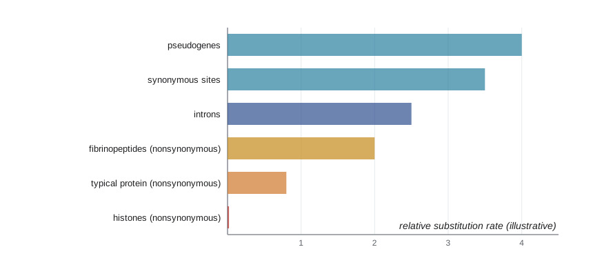
Neutral theory does not deny that adaptive changes happen; it claims that they are a minority of molecular changes and that most variation within species is neutral. In 1973, Tomoko Ohta extended the idea to the nearly neutral theory, which recognizes that many mutations are slightly harmful. In small populations, where N_e s is small, these slightly harmful mutations behave as if neutral and can be fixed; in large populations, selection removes them. The nearly neutral theory explains why some molecular clocks run at different rates in species with different population sizes and generation times.
Testing for selection with neutral theory
Because neutral theory makes precise predictions, it serves as a null hypothesis: departures from it are evidence of selection. One widely used comparison is the ratio of non-synonymous to synonymous substitution rates, dN/dS, often written ω. If amino acid changes are neutral, ω ≈ 1. Purifying selection, which removes harmful amino acid changes, makes ω less than 1, and most genes have ω well below 1. Positive selection, which repeatedly favors new amino acids, can make ω greater than 1. Genes with ω above 1 include those in arms races with pathogens, such as antiviral genes and HLA binding sites, and those involved in reproduction.
# The McDonald–Kreitman test compares polymorphism (within species) with divergence (between species)
# Invented counts for a gene compared between two fruit fly species
from scipy.stats import fisher_exact
Pn, Ps = 2, 42     # non-synonymous and synonymous polymorphisms within species
Dn, Ds = 7, 17     # non-synonymous and synonymous fixed differences between species
odds, pval = fisher_exact([[Dn, Ds], [Pn, Ps]])
alpha = 1 - (Ds*Pn)/(Dn*Ps)    # estimated proportion of substitutions fixed by positive selection
print(f"Dn/Ds = {Dn/Ds:.2f}, Pn/Ps = {Pn/Ps:.2f}")
print(f"Fisher exact test p = {pval:.4f}; estimated alpha = {alpha:.2f}")Dn/Ds = 0.41, Pn/Ps = 0.05 Fisher exact test p = 0.0073; estimated alpha = 0.88
The McDonald–Kreitman test, introduced in 1991 using the Adh gene of fruit flies, compares the ratio of non-synonymous to synonymous changes within a species with the same ratio for fixed differences between species. Under neutrality the two ratios should be equal. In the invented example, amino acid changes make up a much larger share of fixed differences than of polymorphisms, which suggests that many fixed amino acid changes were driven by positive selection; the estimate alpha is the proportion of substitutions that were adaptive. Genome-wide studies using this approach suggest that in fruit flies roughly half of amino acid substitutions were adaptive, while in humans, with a smaller long-term effective size, the proportion is much lower. Methods that use the full distribution of allele frequencies and patterns of linked variation, covered in BIOL-322 and BIOL-410, extend these tests.
Common mistakes
MistakeDrift only matters in tiny populations.
InsteadDrift acts in every finite population; its strength scales with 1/N_e, and N_e is often much smaller than census size.
MistakeDrift tends to favor the more common allele.
InsteadDrift is unbiased: each allele’s chance of fixation equals its current frequency.
MistakeA beneficial mutation will almost certainly spread.
InsteadA new mutation with advantage s is fixed with probability of only about 2s; most are lost by chance.
MistakeEffective population size is the number of individuals counted.
InsteadN_e is the size of an ideal population with the same rate of drift, usually much smaller than the census count.
MistakeNeutral theory says natural selection is unimportant.
InsteadIt says most molecular changes are neutral; adaptive changes still occur and are tested against the neutral expectation.
MistakeA dN/dS ratio below 1 means a gene is not under selection.
InsteadIt indicates purifying selection removing harmful amino acid changes.
Summary and key terms
- Genetic drift is random change in allele frequencies caused by sampling in finite populations.
- Heterozygosity declines by about 1/(2N_e) per generation, and an allele’s chance of fixation equals its frequency.
- Effective population size is reduced by unequal sex ratios, fluctuating size (harmonic mean) and variable family size.
- Bottlenecks and founder effects leave lasting signatures of low diversity and high frequencies of particular alleles.
- A new neutral mutation is fixed with probability 1/(2N); a new beneficial one with probability about 2s; N_e s decides whether drift or selection dominates.
- Neutral theory predicts that the substitution rate equals the mutation rate, explaining the molecular clock and faster evolution of less constrained sequences.
- dN/dS ratios and the McDonald–Kreitman test use neutral expectations to detect purifying and positive selection.
- genetic drift
- Random change in allele frequencies due to sampling in a finite population.
- Wright–Fisher model
- An idealized model in which each generation is a random sample of gene copies from the last.
- heterozygosity
- The probability that two randomly chosen gene copies are different alleles.
- effective population size
- The size of an ideal population that would experience the same rate of drift.
- bottleneck
- A sharp, temporary reduction in population size.
- founder effect
- Loss of variation and change in allele frequencies when a new population is started by a few individuals.
- fixation probability
- The probability that an allele eventually reaches a frequency of 1.
- neutral theory
- Kimura’s theory that most molecular substitutions are selectively neutral and fixed by drift.
- nearly neutral theory
- Ohta’s extension recognizing slightly deleterious mutations whose fate depends on population size.
- dN/dS
- The ratio of non-synonymous to synonymous substitution rates, used to infer selection.
Practice problems
Work each problem on paper first, then reveal the answer to check.
What fraction of heterozygosity does a population with N_e = 100 lose per generation?
Show answer
About 1/200 = 0.5 percent.
An allele has frequency 0.3 and is neutral. What is its probability of eventual fixation?
Show answer
0.3.
A population has 10 breeding males and 90 breeding females. What is N_e?
Show answer
4 × 10 × 90 / 100 = 36.
A population had sizes 500, 50 and 500 in three generations. What is its effective size?
Show answer
1/N_e = (1/3)(0.002 + 0.02 + 0.002) = 0.008, so N_e = 125.
What is the approximate fixation probability of a new mutation with s = 0.02 in a large population?
Show answer
About 2s = 0.04.
Why does the neutral substitution rate not depend on population size?
Show answer
More mutations arise in a larger population (2Nμ), but each is less likely to fix (1/2N); the effects cancel.
Which evolve faster, synonymous or non-synonymous sites, and why?
Show answer
Synonymous sites, because most changes there do not alter the protein and face less purifying selection.
What does ω greater than 1 suggest?
Show answer
Positive selection favoring repeated amino acid changes.
In the McDonald–Kreitman test, what pattern indicates adaptive evolution?
Show answer
A higher ratio of non-synonymous to synonymous changes among fixed differences than among polymorphisms.
Why are some genetic diseases common in populations descended from small groups of founders?
Show answer
Founder effects can raise the frequency of an allele carried by one of the founders.
Lesson quiz · 5 questions
Score 60% or more to complete this lesson.
Create a free account to save your progress, take quizzes and earn a certificate.