The lab scope: voltage, time and triggering

Marty sets a digital storage oscilloscope on Kiran's bench, the four-channel automotive scope the shop bought last spring, and connects one lead to a battery and the other to a small electric motor on the training board. The trace on the screen is not a line but a row of small teeth, one for each brush passing a commutator segment. "A multimeter tells you a number," he says. "A scope tells you a story. It draws voltage against time, so you can see what happens in a millisecond that a meter averages away. Every lesson from here on uses it."

This lesson explains how a lab scope works and how to set it up: what the screen shows, the vertical and horizontal settings, triggering, coupling, sample rate and why too slow a sample rate lies, probes and leads and how to connect them safely, and how to measure frequency and duty cycle. The working example is the purge solenoid on Hal Osei's courier van 2, which Kiran checks against the scan tool's command.

What a scope draws

An oscilloscope draws a graph of voltage, on the vertical axis, against time, on the horizontal axis. A digital storage oscilloscope, which is what every modern automotive scope is, measures the voltage many thousands or millions of times per second, stores the measurements in memory and draws them on a screen. The stored data can be frozen, zoomed, measured and saved. Many automotive scopes are modules connected to a laptop or tablet; others are handheld. All of them do the same basic job.

The screen is divided into a grid of divisions, usually ten across and eight or ten high. The vertical setting, in volts per division, decides how many volts each grid square represents. The horizontal setting, the time base, in seconds or milliseconds per division, decides how much time each square represents. A setting of 2 volts per division with eight divisions shows 16 volts top to bottom; a time base of 10 milliseconds per division with ten divisions shows 100 milliseconds across. Choosing these two settings is the first skill of using a scope.

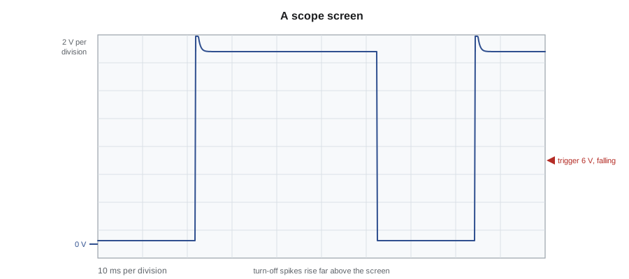
A useful rule for the starting setup is to set the vertical scale so the largest expected voltage fills most of the screen, and the time base so two to five cycles of a repeating signal are visible. For a 12-volt circuit, 2 or 5 volts per division works; for an oxygen sensor that swings between 0.1 and 0.9 volts, 200 millivolts per division. The time base depends on the signal: tens of milliseconds for a solenoid switched a few times a second, a few milliseconds for an injector, and hundreds of milliseconds or seconds for an oxygen sensor.

Triggering: making the picture stand still

A repeating signal drawn continuously would scroll across the screen like a moving train. The trigger makes it stand still by telling the scope to start each sweep at the same point in the signal: when the voltage crosses a chosen trigger level, in a chosen direction, rising or falling, called the slope. Each new sweep starts at the same place in the cycle, so the picture is stable. The trigger point can be placed at the left of the screen or anywhere across it; placing it in the middle shows what happened before as well as after the trigger.

Scopes have trigger modes. In auto mode, the scope sweeps even without a trigger event, which is useful for finding a signal at first. In normal mode, it sweeps only when the trigger condition happens, so the screen holds the last good capture and shows nothing new if the signal stops. In single mode, it captures once and stops, which is how a technician catches a one-off event such as a dropout. Kiran learns to start in auto, set up the vertical scale and time base, then switch to normal and set the trigger level about halfway up the signal on the edge she cares about.

Coupling, ground and channels

DC coupling shows the whole voltage, including its steady level; AC coupling blocks the steady level and shows only the changing part. Most automotive work uses DC coupling, because the actual voltage level matters: a sensor signal that switches between 0.5 and 4.5 volts is very different from one that switches between 2.5 and 4.5. AC coupling is useful for seeing a small ripple on a large voltage, such as the alternator ripple measured in the electrical course, where the ripple is a fraction of a volt riding on about 14 volts.

Each channel has a zero marker on the screen showing where zero volts is drawn. Every voltage is measured relative to the channel's ground lead. On most automotive scopes all channels share a common ground, connected to the vehicle's chassis or battery negative. That means the ground lead must go to a good ground, and the scope cannot measure a voltage between two points that are both above ground, such as across a resistor in the middle of a circuit, by putting the ground lead on one side: doing so connects that point to ground through the scope and can damage the scope or the vehicle. To measure the drop across a component, a technician uses two channels and the scope's math function to subtract one from the other.

Sample rate and aliasing

A digital scope does not see the signal continuously; it samples it. The sample rate is how many measurements per second it takes. The scope chooses the sample rate from the time base and its memory depth, the number of samples it can store per capture. A long time base spreads the same number of samples over more time, so the sample rate falls. If the sample rate falls too low for the signal, the scope cannot draw it correctly. Short spikes can fall between samples and disappear, and a fast repeating signal can appear as a slower one that is not really there. That false picture is called aliasing.

The rule from sampling theory is that a scope needs more than two samples per cycle of the fastest part of a signal just to detect its frequency, and in practice ten or more samples per cycle to draw its shape. The following code shows what happens when a 1,000 hertz signal is sampled too slowly.

# Aliasing: the frequency a scope appears to show when the sample rate is too low
signal_hz = 1000
for rate in (20000, 5000, 2500, 1900, 1100, 1000):
    nyquist = rate / 2
    # the apparent frequency folds back below half the sample rate
    f = signal_hz % rate
    apparent = f if f <= nyquist else rate - f
    shape = "shape drawn well" if rate >= 10 * signal_hz else ("frequency correct, shape crude" if rate > 2 * signal_hz else "FALSE picture")
    print(f"sample rate {rate:6} per second: appears as {apparent:5.0f} Hz  ({shape})")

sample rate  20000 per second: appears as  1000 Hz  (shape drawn well)
sample rate   5000 per second: appears as  1000 Hz  (frequency correct, shape crude)
sample rate   2500 per second: appears as  1000 Hz  (frequency correct, shape crude)
sample rate   1900 per second: appears as   900 Hz  (FALSE picture)
sample rate   1100 per second: appears as   100 Hz  (FALSE picture)
sample rate   1000 per second: appears as     0 Hz  (FALSE picture)

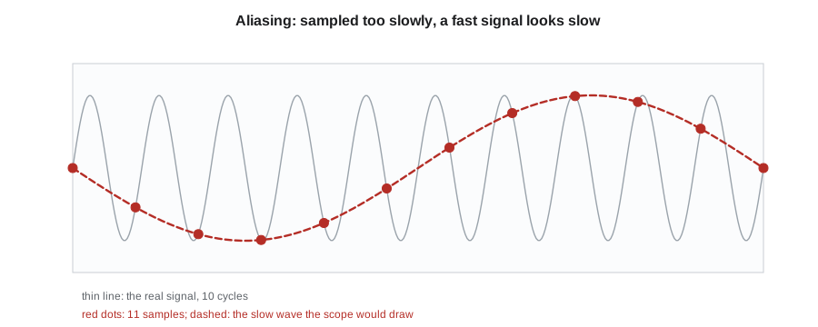
At 1,100 samples per second, the 1,000 hertz signal appears as a 100 hertz signal, and at exactly 1,000 samples per second it appears as a flat line, as if nothing were there. Nothing on the screen warns the technician. Kiran's rule, from Marty: when a waveform looks odd, shorten the time base or increase the sample rate, and see whether the picture changes. A real signal keeps its shape; an alias changes.

Probes, leads and safe connections

Automotive scopes come with test leads, back-probe pins, piercing probes, alligator clips and, for higher voltages, attenuators that divide the voltage by 10 or 20 so the scope can measure it safely. Ignition secondary voltage, which can exceed 30,000 volts, is never connected directly; it is measured with a capacitive pickup clamped around the plug wire or a probe over the coil. Hybrid and electric vehicle high-voltage circuits are measured only with tools rated for them and only by qualified people, as the hybrid course will explain; nothing in this course touches them.

Back-probing means sliding a thin pin into the back of a connector, alongside the wire, until it touches the terminal, without damaging the seal. It lets the technician measure a circuit while it is working. Piercing probes push a needle through the insulation and should be used only where the manufacturer allows, and the hole must be sealed afterward, because a pierced wire lets moisture in and causes corrosion like the fretting Kiran found in Lesson 4. Every lead must be routed away from moving parts, hot exhaust and the cooling fan before the engine is started.

Measuring frequency, duty cycle and peak voltage

Many actuators are switched on and off rapidly to control them. The module turns the circuit on and off a fixed number of times per second, the frequency, and varies the fraction of each cycle that it is on, the duty cycle. Purge solenoids, idle valves on older engines, variable valve timing solenoids, fuel pump drivers and cooling fan modules are controlled this way. On a low-side controlled solenoid, the module switches the ground: when the module turns it on, the scope connected to the ground side reads near zero volts; when it turns it off, the voltage rises to battery voltage, often with a spike from the coil's magnetic field collapsing. The on time is the low part of the waveform.

Hal's van 2 has a faint ticking under the hood and a fuel smell after refueling. The scan tool shows the purge solenoid commanded at 35 percent. Kiran back-probes the solenoid's control wire, the ground side, sets 5 volts per division and 20 milliseconds per division, and triggers on the falling edge at 6 volts. The waveform is clean and regular. She exports a short capture and runs it through the shop's analysis script.

# Measure frequency, duty cycle and peak voltage from a sampled low-side solenoid waveform
import math
rate = 10000                         # samples per second
f_cmd, duty_cmd, vbat = 16.0, 0.35, 13.8
samples = []
for i in range(int(rate * 0.25)):    # a quarter of a second of signal
    t = i / rate
    phase = (t * f_cmd) % 1.0
    if phase < duty_cmd:
        v = 0.25                     # transistor on: circuit pulled to ground
    else:
        since_off = (phase - duty_cmd) / f_cmd
        v = vbat + 46.0 * math.exp(-since_off / 0.0002)   # inductive spike decays at turn-off
    samples.append(v)
threshold = vbat / 2
falls = [i for i in range(1, len(samples)) if samples[i - 1] > threshold >= samples[i]]
period = (falls[-1] - falls[0]) / (len(falls) - 1) / rate
low = sum(1 for v in samples[falls[0]:falls[-1]] if v < threshold)
duty = low / (falls[-1] - falls[0])
print(f"frequency: {1 / period:.1f} Hz")
print(f"on time (low): {duty * period * 1000:.1f} ms of each {period * 1000:.1f} ms, duty cycle {duty:.0%}")
print(f"peak voltage at turn-off: {max(samples):.1f} V")

frequency: 16.0 Hz
on time (low): 21.9 ms of each 62.5 ms, duty cycle 35%
peak voltage at turn-off: 54.4 V

The scope measures 16 hertz and a duty cycle of 35 percent, matching the command, and a turn-off spike of about 54 volts, which shows the solenoid's coil is intact: a coil with shorted turns or an open winding would produce a much smaller spike or none. The solenoid is being controlled correctly. Kiran now has to find out why the van smells of fuel after refueling, which is an EVAP question the emissions course already taught her to answer. She smoke-tests the EVAP system and finds the purge solenoid's internal valve leaking past its seat when it is commanded closed, which lets the fuel tank's vapor flow into the intake during refueling with the engine off. A solenoid can be electrically perfect and mechanically faulty; the scope proved the first, the smoke test the second.

Scope or multimeter?

A multimeter is the right tool for steady voltages, resistances and voltage drops, and for most quick checks. A scope is the right tool whenever the signal changes quickly: switching actuators, pulse or frequency signals from sensors, network signals, dropouts and glitches, and anything where the shape of the signal matters. A multimeter averages a switching signal into a single number that can be misleading: on the purge solenoid's control wire, a meter would show about 9 volts, which looks like a fault but is just the average of 0.25 and 13.8 volts weighted by the duty cycle.

# What a multimeter shows on a switching signal: the average, which can mislead
vbat, v_on, duty = 13.8, 0.25, 0.35
average = v_on * duty + vbat * (1 - duty)
print(f"duty cycle {duty:.0%}: scope shows {v_on} V and {vbat} V; a meter shows about {average:.1f} V")

duty cycle 35%: scope shows 0.25 V and 13.8 V; a meter shows about 9.1 V

Kiran adds one more habit: before trusting a scope on an unknown circuit, she checks it on a known one. A quick capture of the battery voltage with the engine running, which should show a steady 14 volts with a small alternator ripple, proves the leads, the ground and the settings are working.