Impossibility results and fairness trade-offs

Lesson 3 introduced several reasonable definitions of fairness. A natural hope is to find a classifier that satisfies all of them. Unfortunately, a set of results published in 2016 and 2017 showed that this is impossible except in special cases. When groups have different base rates, a classifier cannot simultaneously be calibrated within groups and have equal false positive and false negative rates, unless it predicts perfectly. These impossibility theorems explain the COMPAS debate, in which two sides drew opposite conclusions from the same data, and they force practitioners to make explicit choices. This lesson explains the results, demonstrates them in code, and discusses how to reason about the trade-offs among fairness criteria and between fairness and accuracy.

The COMPAS debate

In 2016 ProPublica analyzed the COMPAS risk assessment tool used in US courts to predict whether defendants would reoffend. It found that among defendants who did not reoffend, Black defendants were labeled higher risk about 45 % of the time against 23 % for white defendants, while among those who did reoffend, white defendants were more often labeled low risk. The company that developed the tool responded that its scores were calibrated: at each risk level, Black and white defendants reoffended at similar rates, and so a high-risk label meant the same thing for both groups. Researchers quickly showed that both statements could be true at once, and that this was not a peculiarity of COMPAS but a mathematical necessity whenever base rates differ.

The impossibility theorem

Kleinberg, Mullainathan and Raghavan proved that three conditions cannot hold together unless the groups have equal base rates or prediction is perfect: calibration within groups, balance for the positive class (equal average score among people with \(Y=1\)) and balance for the negative class (equal average score among people with \(Y=0\)). Chouldechova proved a related result for binary predictions using a simple identity linking the false positive rate, the false negative rate, the positive predictive value and the base rate \(p\) of a group:

If two groups have the same PPV (predictive parity) and the same FNR but different base rates \(p\), the identity forces their FPRs to differ. Equalizing FPR and FNR instead forces PPVs to differ. There is no escape short of equal base rates or a perfect classifier. Which constraint to give up is therefore a choice about which kind of unfairness matters most in the context.

Seeing it in code

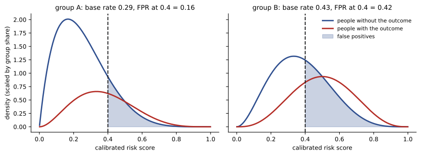
The following simulation gives each person a true risk drawn from a group-specific distribution, with group B having higher average risk. The score is the true risk itself, so it is perfectly calibrated for both groups by construction. We then apply common thresholds and measure error rates.

import numpy as np
# A calibrated score with different base rates cannot equalize error rates
rng = np.random.default_rng(4)
n = 200_000
group = rng.choice(["A", "B"], n)
# each person has a true risk p; the score equals p, so it is perfectly calibrated in both groups
p = np.where(group == "A", rng.beta(2, 5, n), rng.beta(3, 4, n))    # group B has higher average risk
y = rng.random(n) < p
print("calibration check (mean outcome within score bins)")
print("bin        A      B")
for lo in (0.1, 0.3, 0.5, 0.7):
    m = (p >= lo) & (p < lo + 0.1)
    a = y[m & (group == "A")].mean(); b = y[m & (group == "B")].mean()
    print(f"{lo:.1f}-{lo + 0.1:.1f}   {a:.2f}   {b:.2f}")
print()
print("threshold  FPR_A  FPR_B  FNR_A  FNR_B  PPV_A  PPV_B")
for t in (0.3, 0.4, 0.5):
    out = []
    for g in ("A", "B"):
        m = group == g; pr = p[m] >= t; yy = y[m]
        out.append((pr[~yy].mean(), 1 - pr[yy].mean(), yy[pr].mean()))
    (fa, na, pa), (fb, nb, pb) = out
    print(f"{t:9.1f}  {fa:.2f}   {fb:.2f}   {na:.2f}   {nb:.2f}   {pa:.2f}   {pb:.2f}")
base_a, base_b = y[group == "A"].mean(), y[group == "B"].mean()
print(f"base rates: A {base_a:.2f}, B {base_b:.2f}")

calibration check (mean outcome within score bins)
bin        A      B
0.1-0.2   0.15   0.16
0.3-0.4   0.34   0.35
0.5-0.6   0.54   0.54
0.7-0.8   0.74   0.75

threshold  FPR_A  FPR_B  FNR_A  FNR_B  PPV_A  PPV_B
      0.3  0.33   0.65   0.35   0.13   0.44   0.50
      0.4  0.16   0.42   0.58   0.29   0.51   0.56
      0.5  0.06   0.23   0.78   0.50   0.58   0.62
base rates: A 0.29, B 0.43

The calibration check confirms that within each score bin, the outcome rate is the same for both groups and matches the score. Yet at every threshold, group B has a much higher false positive rate (0.42 against 0.16 at threshold 0.4) and a much lower false negative rate (0.29 against 0.58). Precision is also slightly higher for B. Nothing about the score treats the groups differently: a person with risk 0.45 is treated the same whatever their group. The disparity in error rates comes entirely from the different distributions of risk, which put more of group B's negatives above the threshold. This is exactly the COMPAS pattern, and it shows why calibration and equalized odds pull in different directions.

Achieving equalized odds

If a context calls for equal error rates, we can use group-specific thresholds or randomized decisions near the threshold. Hardt, Price and Srebro showed that any score can be post-processed into a classifier satisfying equalized odds by choosing, for each group, a point on its ROC curve where the two groups' curves intersect, possibly mixing two thresholds randomly. The cost is that the resulting decisions are no longer calibrated: a given score leads to different decisions for different groups, which some consider unfair in itself and which may be legally restricted in some domains (Lesson 5). Equal opportunity, which only requires equal true positive rates, is easier to achieve with less accuracy loss.

Fairness and accuracy

Imposing a fairness constraint usually reduces accuracy measured against the available labels, because the unconstrained model is by definition the most accurate one under those labels. The size of the cost varies: it is often small, since many models have room to move along a flat region of the accuracy surface, but it can be large if the constraint fights strong signal in the data. Two caveats matter. First, accuracy against biased labels is not the same as accuracy against the truth: if labels under-record the qualifications of one group, a fairness constraint can improve true accuracy, as Lesson 5 demonstrates. Second, many equally accurate models can differ greatly in fairness, a phenomenon called the Rashomon effect or model multiplicity. Searching among near-optimal models for the fairest one often finds large fairness gains at almost no accuracy cost.

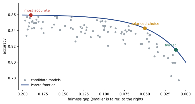
The Pareto frontier

Trade-offs are best visualized as a Pareto frontier: for each level of a fairness metric, the best achievable accuracy. Points on the frontier are not dominated by any other model; points below it can be improved in both respects. Plotting candidate models, thresholds or mitigation strengths against accuracy and fairness metrics gives decision-makers a concrete menu of options instead of an abstract debate. The choice of where to sit on the frontier is a policy decision, best made with stakeholders who understand the consequences of each kind of error.

Thinking about costs

A structured way to choose is to assign costs to each kind of error for each group and to consider who bears them. In lending, a false negative denies credit to someone who would repay, harming the applicant; a false positive lends to someone who will default, harming both the lender and, through debt, the borrower. In child welfare screening, a false positive subjects a family to an intrusive investigation, while a false negative may leave a child at risk. Making these costs explicit, and asking whether they fall disproportionately on groups already disadvantaged, helps decide whether to equalize false positive rates, false negative rates, or precision.

Beyond the classifier

Impossibility results concern a classifier in isolation. Often the most effective response is to change the decision process: gather better information so predictions become more accurate for everyone, change the intervention so that a false positive is less harmful (offering support rather than imposing penalties), or address the causes of different base rates. Fairness is a property of the whole socio-technical system, not only of the model.

A worked threshold choice

Consider a screening tool for a scholarship program with limited places. The developers compute selection rates, true positive rates and precision for two groups at thresholds from 0.3 to 0.7 and lay the results out in a table alongside overall accuracy. At 0.5, the tool is calibrated, but qualified applicants from the group with fewer historical opportunities are selected less often. Lowering that group's threshold to 0.45 equalizes true positive rates and costs one percentage point of accuracy against the available labels. The committee, which includes former scholarship recipients, decides that missing qualified applicants is the more serious harm in this context and that the program's purpose is to widen access, so it adopts equal opportunity as its criterion, records the reasoning and the accuracy cost, and commits to review the outcomes of selected students after one year. Another committee in a different context, say a medical test where false positives lead to invasive procedures, might reasonably decide differently.

The example shows the pattern the impossibility results demand: compute the alternatives, make the trade-off visible, decide with people who understand the stakes, and document the choice so that it can be revisited.

Fairness over time

Most fairness criteria are static: they compare groups at a single point. Decisions, however, have long-term effects. Liu and colleagues showed that imposing demographic parity on lending can, under some conditions, harm the group it is meant to help, if loans are extended to applicants who then default and see their credit scores fall. Conversely, denying opportunities can entrench disadvantage, because people who are never given a loan never build a credit history. Simulation studies of these delayed effects, combined with monitoring of outcomes after deployment (Lesson 12), help assess whether a fairness intervention improves people's situations over time or only improves a metric at launch.