Diffusion and multimodal models

Generative AI is not only text. Since 2022, models that create images from text descriptions, such as DALL-E, Midjourney, Stable Diffusion, Imagen and Flux, have reached photographic quality, and video models such as Sora and Veo now generate short clips with sound. At the same time, language models have become multimodal: they read images, charts, documents and audio, and some generate images and speech directly. This lesson explains diffusion models, the main technology behind image and video generation; how text conditions them; latent diffusion and diffusion transformers; how multimodal language models combine vision and text; and the questions of provenance, deepfakes and copyright that these capabilities raise.

Generative models before diffusion

A generative model learns to produce new samples that resemble its training data. Earlier approaches include variational autoencoders (VAEs, 2013), which encode data into a compressed latent space and decode samples from it, but tend to produce blurry images; and generative adversarial networks (GANs, 2014), in which a generator tries to fool a discriminator that distinguishes real from generated images. GANs produced sharp faces and scenes by the late 2010s but were unstable to train and tended to cover only part of the data's variety (mode collapse). Autoregressive models generated images pixel by pixel or token by token, which was slow for large images. Diffusion models, popularized from 2020, combine stable training, high quality and broad coverage, and became the dominant approach for images, video and audio.

The forward process: adding noise

A diffusion model is built around two processes. The forward process gradually destroys data by adding small amounts of Gaussian noise over many steps \(t = 1, \dots, T\), until nothing but noise remains. With a noise schedule \(\beta_t\), each step is:

A convenient property is that the noisy sample at any step can be produced directly from the clean data in one jump, using the cumulative product \(\bar{\alpha}_t = \prod_{s \le t} (1 - \beta_s)\):

import numpy as np

T = 1000
betas = np.linspace(1e-4, 0.02, T)
alpha_bar = np.cumprod(1 - betas)
for t in [1, 100, 250, 500, 750, 1000]:
    ab = alpha_bar[t - 1]
    print(f"t={t:>4}  signal scale {np.sqrt(ab):.3f}  noise scale {np.sqrt(1 - ab):.3f}  SNR {ab / (1 - ab):10.4f}")

rng = np.random.default_rng(0)
x0 = np.full(20000, 2.0)
x = x0.copy()
for t in range(500):
    x = np.sqrt(1 - betas[t]) * x + np.sqrt(betas[t]) * rng.normal(size=x.size)
direct = np.sqrt(alpha_bar[499]) * x0 + np.sqrt(1 - alpha_bar[499]) * rng.normal(size=x0.size)
print(f"after 500 steps: step-by-step mean {x.mean():.3f} std {x.std():.3f};  closed form mean {direct.mean():.3f} std {direct.std():.3f}")

t=   1  signal scale 1.000  noise scale 0.010  SNR  9999.0000
t= 100  signal scale 0.947  noise scale 0.321  SNR     8.7104
t= 250  signal scale 0.724  noise scale 0.690  SNR     1.1012
t= 500  signal scale 0.280  noise scale 0.960  SNR     0.0853
t= 750  signal scale 0.058  noise scale 0.998  SNR     0.0034
t=1000  signal scale 0.006  noise scale 1.000  SNR     0.0000
after 500 steps: step-by-step mean 0.555 std 0.962;  closed form mean 0.553 std 0.959

The signal-to-noise ratio \(\bar{\alpha}_t / (1 - \bar{\alpha}_t)\) falls from very high to essentially zero, so the final \(x_T\) is indistinguishable from pure noise.

The reverse process: learning to denoise

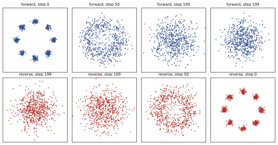
Generation runs the process backwards: start from pure noise and remove a little noise at a time until a clean sample appears. The model, a neural network \(\epsilon_\theta(x_t, t)\), is trained to predict the noise that was added to a noisy sample. The training procedure (from the 2020 DDPM paper by Ho, Jain and Abbeel) is remarkably simple: take a training image, pick a random step \(t\), add noise with the one-jump formula, and train the network to predict that noise with a mean squared error loss:

Predicting the noise is equivalent to estimating the score, the gradient of the log probability density of the noisy data, which points toward regions where data is more likely. Sampling uses the predicted noise to take a small step toward the data at each step:

where \(z\) is fresh noise (omitted at the last step). The original method needed about 1,000 network evaluations per image; later samplers (DDIM, higher-order ODE solvers) and distillation methods cut this to tens or even a few steps.

import numpy as np

rng = np.random.default_rng(0)
K = 8
angles = 2 * np.pi * np.arange(K) / K
mu = 2 * np.column_stack([np.cos(angles), np.sin(angles)])
s2 = 0.02
T = 200
betas = np.linspace(1e-4, 0.05, T)
alphas = 1 - betas
ab = np.cumprod(alphas)


def eps_hat(x, t, comps):
    m = np.sqrt(ab[t]) * mu[comps]
    v = ab[t] * s2 + 1 - ab[t]
    d2 = ((x[:, None, :] - m[None]) ** 2).sum(-1)
    w = np.exp(-(d2 - d2.min(1, keepdims=True)) / (2 * v))
    w /= w.sum(1, keepdims=True)
    score = (w[:, :, None] * (m[None] - x[:, None, :])).sum(1) / v
    return -np.sqrt(1 - ab[t]) * score


def sample(n, guidance=0.0, cond=None):
    x = rng.normal(size=(n, 2))
    allc = np.arange(K)
    for t in reversed(range(T)):
        e = eps_hat(x, t, allc)
        if cond is not None:
            e = (1 + guidance) * eps_hat(x, t, cond) - guidance * e
        mean = (x - betas[t] / np.sqrt(1 - ab[t]) * e) / np.sqrt(alphas[t])
        x = mean + (np.sqrt(betas[t]) * rng.normal(size=x.shape) if t > 0 else 0)
    return x


x = sample(2000)
nearest = np.argmin(((x[:, None] - mu[None]) ** 2).sum(-1), 1)
dist = np.sqrt(((x - mu[nearest]) ** 2).sum(1))
print("unconditional: samples per mode", np.bincount(nearest, minlength=K), f" median distance to mode {np.median(dist):.3f}")
left = np.array([3, 4, 5])
for g in [0.0, 1.0, 3.0]:
    x = sample(2000, g, left)
    nearest = np.argmin(((x[:, None] - mu[None]) ** 2).sum(-1), 1)
    dist = np.sqrt(((x - mu[nearest]) ** 2).sum(1))
    counts = np.bincount(nearest, minlength=K)[left]
    print(f"left modes, guidance {g}: share in left {np.isin(nearest, left).mean():.2f}  counts {counts}  median distance {np.median(dist):.3f}")

unconditional: samples per mode [256 246 295 215 219 243 271 255]  median distance to mode 0.174
left modes, guidance 0.0: share in left 1.00  counts [618 688 694]  median distance 0.173
left modes, guidance 1.0: share in left 1.00  counts [544 857 599]  median distance 0.173
left modes, guidance 3.0: share in left 1.00  counts [ 423 1121  456]  median distance 0.174

Because the toy data is a known mixture, the code computes the ideal noise prediction exactly instead of training a network; a real model learns an approximation of this function from data. The unconditional samples cover all eight clusters about equally, showing that diffusion does not suffer from mode collapse.

Conditioning and classifier-free guidance

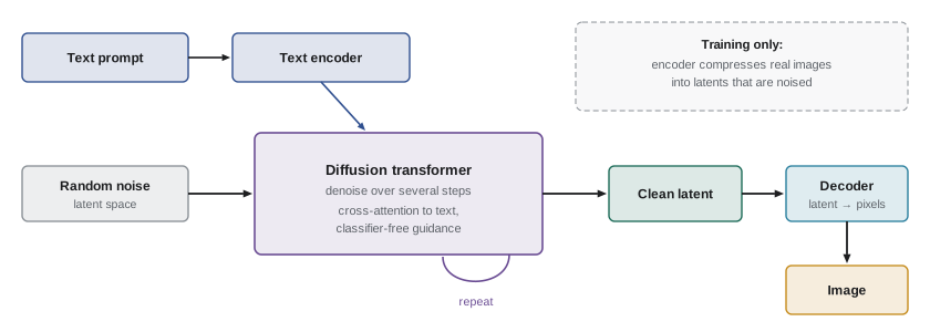
To generate an image from a description, the denoising network is conditioned on an embedding of the text, produced by a text encoder such as CLIP's or a language model's, and injected through cross-attention layers. Classifier-free guidance (Ho and Salimans, 2022) strengthens the effect of the condition. The same network is trained both with the text and, some of the time, without it; at sampling time the two predictions are combined:

where \(c\) is the condition and \(w\) the guidance weight. Larger \(w\) pushes samples toward images that strongly match the prompt, improving prompt adherence and apparent quality at the cost of diversity. The code output shows this: with guidance, samples concentrate on the most typical cluster of the condition instead of spreading over all three. Very high guidance produces oversaturated, stereotyped images.

Latent diffusion and diffusion transformers

Running diffusion directly on high-resolution pixels is expensive. Latent diffusion (Rombach and colleagues, 2022), the basis of Stable Diffusion, first trains an autoencoder that compresses images into a smaller latent representation, for example a 512 × 512 × 3 image into a 64 × 64 × 4 latent (48 times fewer values), and runs diffusion in that latent space. The decoder turns the final latent back into pixels. This made high-quality image generation feasible on consumer GPUs.

The denoising network was originally a U-Net, a convolutional architecture. Since 2023, diffusion transformers (DiT), which split the latent into patches and process them as tokens with a transformer, have taken over in leading models because they scale predictably with compute, much like language models. Many recent models also replace the original diffusion formulation with flow matching (or rectified flow), which trains the network to predict a velocity that moves samples along straighter paths from noise to data, allowing fewer sampling steps. Stable Diffusion 3 and Flux use this approach.

Video models extend the same ideas to sequences of frames, treating video as patches in space and time (spacetime patches). OpenAI's Sora, previewed in February 2024, demonstrated minute-long coherent clips, and Google's Veo 3, released in 2025, added synchronized dialogue and sound. Video generation is far more computationally intensive than images, and maintaining consistency of objects and physics over time remains a challenge. Diffusion and related models also generate audio, music, speech, 3D shapes and even protein structures.

Multimodal language models

Multimodal language models accept images (and sometimes audio and video) along with text. A common design connects a vision encoder, typically a vision transformer pretrained with CLIP-style contrastive learning on image-caption pairs (AI-350), to a language model: the image is split into patches, encoded into vectors, projected into the language model's embedding space, and inserted into the token sequence as "image tokens". The combined model is then trained on image-text data and instruction examples, learning to describe images, read text and charts, answer questions about documents and reason about diagrams. Newer models are natively multimodal, trained from the start on interleaved text, images and audio.

Some multimodal models also generate images or speech. They may call a separate diffusion model, or generate image tokens autoregressively within the same model, an approach that lets image generation follow complex instructions and render text accurately, as shown by several systems released in 2025. Speech-to-speech models process audio tokens directly, enabling spoken conversations with low latency.

Provenance, deepfakes and misuse

Realistic synthetic media can be misused: impersonating people in fraudulent video calls or voice messages, spreading political disinformation, creating non-consensual intimate images, or fabricating evidence. Responses include:

• Provenance standards such as C2PA content credentials, which attach signed metadata describing how an image was created and edited.
• Watermarking, such as Google's SynthID, which embeds imperceptible signals in generated images, audio, video and text that detectors can find.
• Usage policies and safety filters in generation systems that refuse to create certain content, such as sexual images of real people.
• Detection tools, which are useful but imperfect, since generated media keeps improving and metadata can be stripped.
• Law: the federal TAKE IT DOWN Act (2025) makes publishing non-consensual intimate images, including AI-generated ones, a crime and requires platforms to remove them within 48 hours of a valid request; many states also regulate election deepfakes and digital replicas of voices and likenesses.

Copyright and training data

Generative models are trained on large collections of text and images, much of it copyrighted, which has led to lawsuits and policy debate over whether training is lawful and whether outputs infringe.

In the US, courts are applying fair use. In June 2025 two federal judges in California ruled for the AI developers on fair use for training in cases against Anthropic and Meta, on different reasoning; the Anthropic ruling held that building a library from pirated copies was not fair use, and that case later settled for $1.5 billion; earlier in 2025 a court rejected fair use for a non-generative legal research tool trained on Thomson Reuters headnotes. Other cases, including The New York Times against OpenAI and Microsoft, continue. The Copyright Office and courts have held that works need human authorship to be protected, so purely AI-generated images are not copyrightable, while human selection, arrangement and modification can be.

Practical steps for organizations include choosing models whose providers offer indemnities or licensed training data, avoiding prompts that request copies of specific protected works or real people's likenesses, disclosing AI-generated content where appropriate, and keeping humans responsible for what is published.

Lesson 10 returns to contrastive models such as CLIP, which link images and text in many of the systems described here, and Lesson 11 covers the wider safeguards for deployed generative systems.